Labour costs by NACE Rev. 2 activity - lc_an_cost_r2

Data - Eurostat

Info

Last observation: Annual: 2011 (N = 6,483)

First observation: Annual: 1996 (N = 174)

Last data update: 23 jul 2026, 22:37. Last compile: 24 jul 2026, 02:09

Structure

freq

nace_r2

sizeclas

indic_lc

currency

geo

Hourly Labour Cost, Whole Economy

Germany, 1996-2011

lc_an_cost_r2 %>%
  filter(geo == "DE",
         indic_lc == "LC_H",
         currency == "EUR",
         sizeclas == "GE10",
         nace_r2 == "B-S_X_O") %>%
  year_to_date %>%
  ggplot + geom_line(aes(x = date, y = values)) +
  theme_minimal() +
  scale_x_date(breaks = as.Date(paste0(seq(1995, 2100, 2), "-01-01")),
               labels = date_format("%Y")) +
  xlab("") + ylab("Hourly labour cost, Germany (EUR)")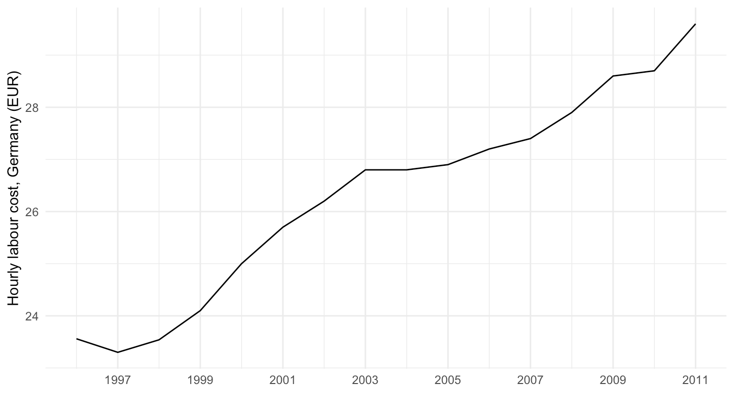

France, Germany, Spain, Italy, Poland, 2008-2011

lc_an_cost_r2 %>%
  filter(geo %in% c("FR", "DE", "ES", "IT", "PL"),
         indic_lc == "LC_H",
         currency == "EUR",
         sizeclas == "GE10",
         nace_r2 == "B-S_X_O",
         time >= "2008") %>%
  year_to_date %>%
  left_join(colors, by = c("Geo" = "country")) %>%
  ggplot + geom_line(aes(x = date, y = values, color = color)) +
  theme_minimal() + scale_color_identity() + add_5flags +
  scale_x_date(breaks = as.Date(paste0(seq(2008, 2100, 1), "-01-01")),
               labels = date_format("%Y")) +
  xlab("") + ylab("Hourly labour cost (EUR)")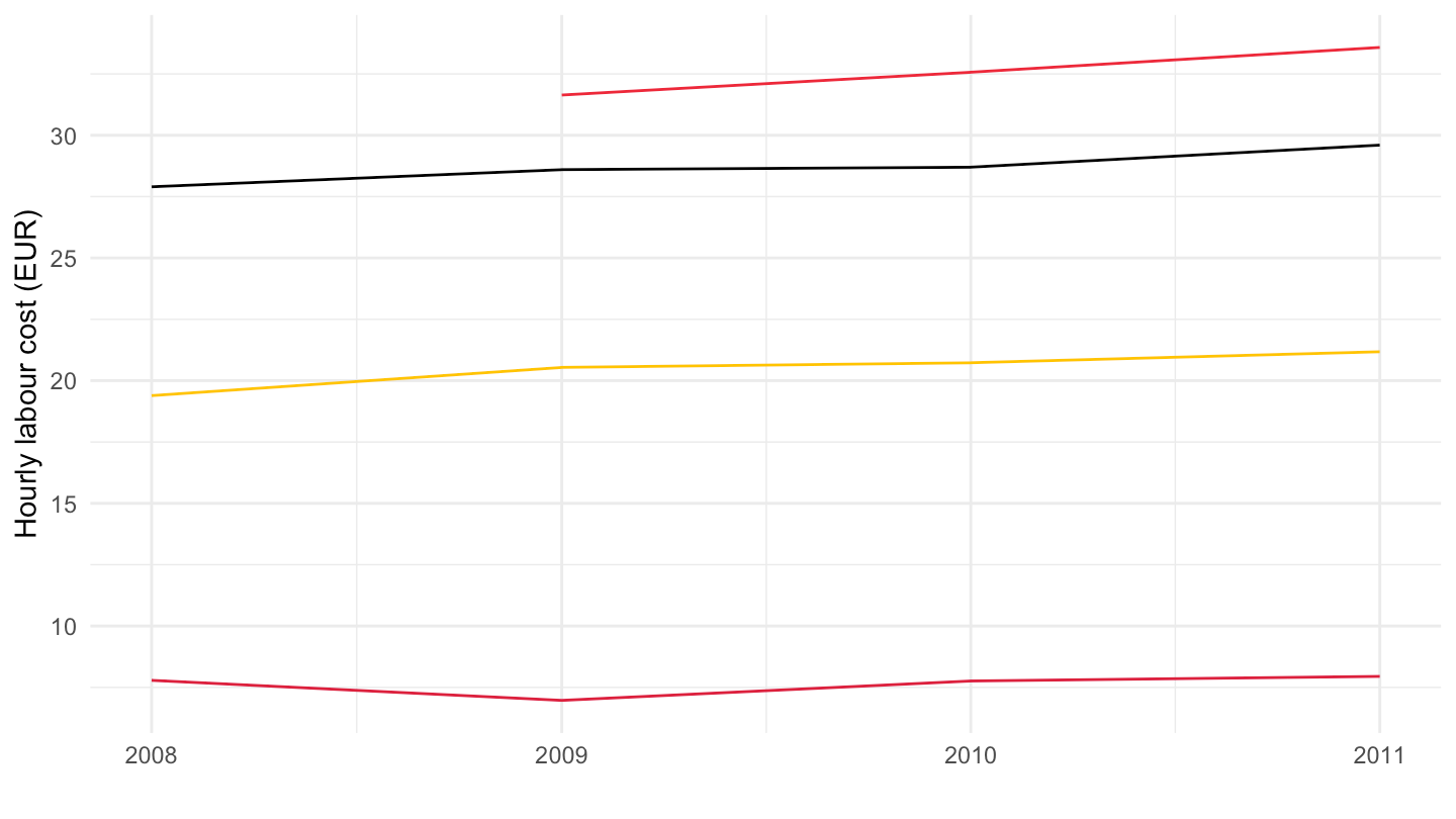

Hourly Labour Cost by Sector, Germany

lc_an_cost_r2 %>%
  filter(geo == "DE",
         indic_lc == "LC_H",
         currency == "EUR",
         sizeclas == "GE10",
         nace_r2 %in% c("C", "F", "G", "K")) %>%
  year_to_date %>%
  ggplot + geom_line(aes(x = date, y = values, color = Nace_r2)) +
  theme_minimal() +
  theme(legend.position = c(0.3, 0.82),
        legend.title = element_blank()) +
  scale_x_date(breaks = as.Date(paste0(seq(1995, 2100, 2), "-01-01")),
               labels = date_format("%Y")) +
  xlab("") + ylab("Hourly labour cost, Germany (EUR)")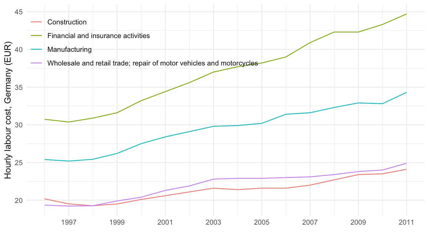

2011 Snapshot: Hourly Labour Cost by Country

latest_y <- lc_an_cost_r2 %>%
  filter(indic_lc == "LC_H", currency == "EUR", sizeclas == "GE10",
         nace_r2 == "B-S_X_O", !is.na(values)) %>%
  summarise(m = max(time)) %>%
  pull(m)

lc_an_cost_r2 %>%
  filter(indic_lc == "LC_H",
         currency == "EUR",
         sizeclas == "GE10",
         nace_r2 == "B-S_X_O",
         time == latest_y,
         !is.na(values)) %>%
  select(Geo, values) %>%
  arrange(desc(values)) %>%
  print_table_conditional()

Geo	values
Denmark	38.35
Sweden	36.42
Belgium	35.72
Luxembourg	33.72
France	33.58
Netherlands	31.92
Germany	29.60
Finland	29.41
Ireland	25.82
Spain	21.18
United Kingdom	19.31
Slovenia	14.90
Portugal	13.01
Czechia	9.92
Croatia	9.16
Slovakia	8.54
Poland	7.95
Hungary	7.17
Lithuania	5.62
Latvia	5.43
Romania	4.18
Bulgaria	3.28