Overcrowding rate by age, sex and poverty status - total population - EU-SILC survey - ilc_lvho05a

Data - Eurostat

Author

François Geerolf

Info

Last observation: 2025 (N = 4736)

First observation: 2003 (N = 1006)

Last data update: 14 aoû 2026, 20:53. Last compile: 18 aoû 2026, 01:34

Structure

France: Overcrowding by Poverty Status

Above vs. Below 60% of Median Income

Code

ilc_lvho05a |>
  filter(geo == "FR",
         age == "TOTAL",
         sex == "T",
         rskpovth != "TOTAL") |>
  year_to_date() |>

  mutate(values = values/100) |>
  ggplot() + geom_line(aes(x = date, y = values, color = Rskpovth)) +
  theme_minimal() +
  scale_x_date(breaks = as.Date(paste0(seq(2000, 2100, 2), "-01-01")),
               labels = date_format("%Y")) +
  theme(legend.position = c(0.8, 0.85),
        legend.title = element_blank()) +
  xlab("") + ylab("Overcrowding rate") +
  scale_y_continuous(labels = scales::percent_format(accuracy = 1))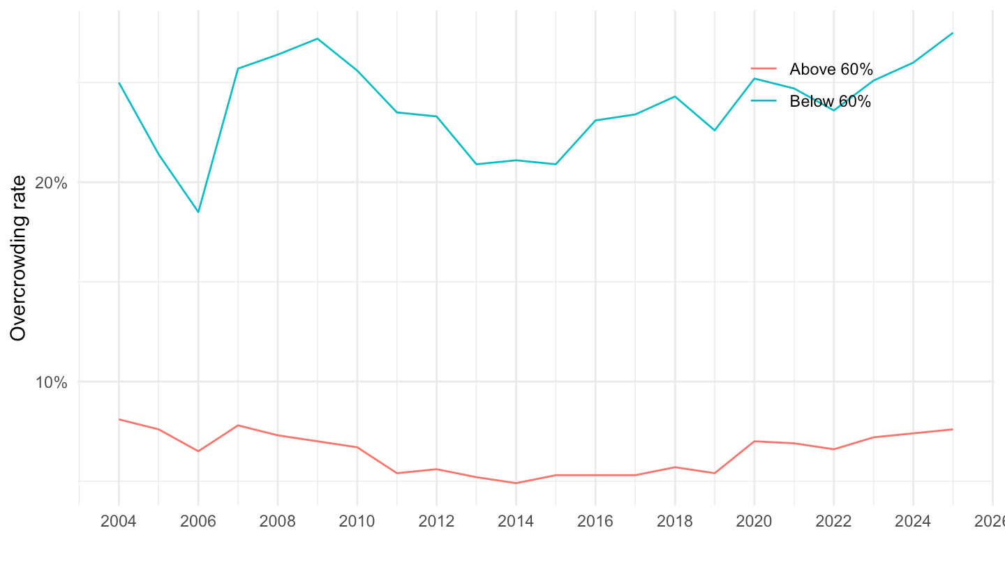

EU27: Overcrowding by Age Group

Children vs. 65 and Over

Code

ilc_lvho05a |>
  filter(geo == "EU27_2020",
         sex == "T",
         rskpovth == "TOTAL",
         age %in% c("Y_LT18", "Y_GE65")) |>
  year_to_date() |>

  mutate(values = values/100) |>
  ggplot() + geom_line(aes(x = date, y = values, color = Age)) +
  theme_minimal() +
  scale_x_date(breaks = as.Date(paste0(seq(2000, 2100, 2), "-01-01")),
               labels = date_format("%Y")) +
  theme(legend.position = c(0.8, 0.15),
        legend.title = element_blank()) +
  xlab("") + ylab("Overcrowding rate") +
  scale_y_continuous(labels = scales::percent_format(accuracy = 1))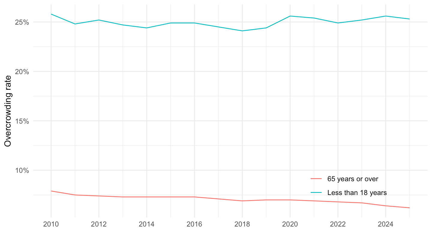

Latest Year by Country

Code

latest_y <- ilc_lvho05a |>
  filter(geo == "EU27_2020",
         age == "TOTAL",
         sex == "T",
         rskpovth == "TOTAL",
         !is.na(values)) |>
  summarise(m = max(time)) |>
  pull(m)

ilc_lvho05a |>
  filter(geo %in% c("EU27_2020", "FR", "DE", "IT", "ES", "NL", "PL", "SE"),
         age == "TOTAL",
         sex == "T",
         rskpovth != "TOTAL",
         time == latest_y) |>
  select(Geo, Rskpovth, values) |>
  spread(Rskpovth, values) |>
  arrange(-`Below 60%`) |>
  print_table_conditional()

Geo	Above 60%	Below 60%
Sweden	11.0	41.2
Poland	29.8	38.2
Italy	21.8	35.2
European Union - 27 countries (from 2020)	14.3	29.8
France	7.6	27.5
Germany	8.8	27.4
Spain	7.4	17.9
Netherlands	2.8	13.4

Overcrowding Rate Over Time (Total Population)

France, Germany, Italy, Spain, Netherlands

Code

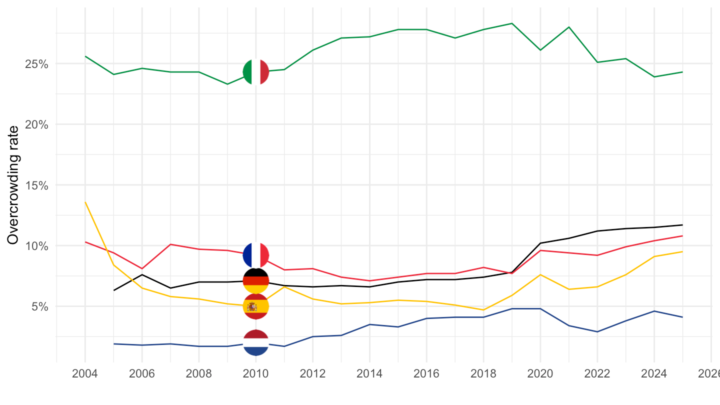
ilc_lvho05a |>
  filter(geo %in% c("FR", "DE", "IT", "ES", "NL"),
         age == "TOTAL",
         sex == "T",
         rskpovth == "TOTAL") |>
  year_to_date() |>

  left_join(colors, by = c("Geo" = "country")) |>
  mutate(values = values/100) |>
  mutate(color = ifelse(geo == "NL", color2, color)) |>
  ggplot() + geom_line(aes(x = date, y = values, color = color)) +
  theme_minimal() + scale_color_identity() + add_flags +
  scale_x_date(breaks = as.Date(paste0(seq(2000, 2100, 2), "-01-01")),
               labels = date_format("%Y")) +
  xlab("") + ylab("Overcrowding rate") +
  scale_y_continuous(breaks = 0.01*seq(0, 60, 5),
                     labels = scales::percent_format(accuracy = 1))