Distribution of population by tenure status, type of household and income group - EU-SILC survey - ilc_lvho02

Data - Eurostat

Author

François Geerolf

Info

Last observation: Annual: 2025 (N = 11,781)

First observation: Annual: 2003 (N = 1,785)

Last data update: 11 aoû 2026, 22:30. Last compile: 12 aoû 2026, 00:37

Structure

France, Germany, Spain, Italy

Share of Homeowners

Code

ilc_lvho02 |>
  filter(geo %in% c("FR", "DE", "ES", "IT"),
         rskpovth == "TOTAL",
         hhcomp == "TOTAL",
         tenure == "OWN") |>
  year_to_date() |>
  left_join(colors, by = c("Geo" = "country")) |>
  mutate(values = values/100) |>
  ggplot() + geom_line(aes(x = date, y = values, color = color)) +
  theme_minimal() + scale_color_identity() + add_flags +
  scale_x_date(breaks = as.Date(paste0(seq(2000, 2100, 2), "-01-01")),
               labels = date_format("%Y")) +
  xlab("") + ylab("Share of population that owns its home") +
  scale_y_continuous(labels = scales::percent_format(accuracy = 1))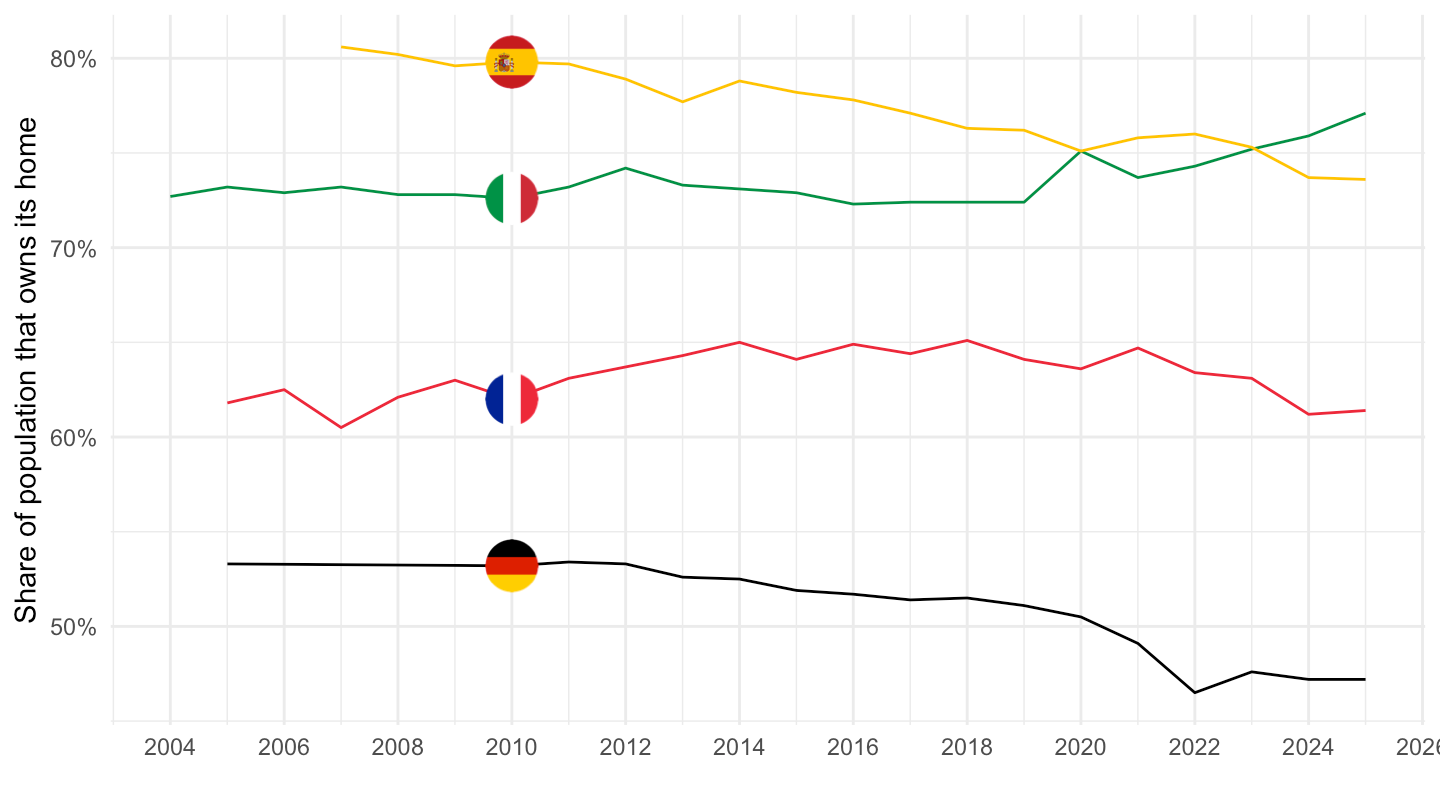

France

Tenure Status Over Time

Code

ilc_lvho02 |>
  filter(geo == "FR",
         rskpovth == "TOTAL",
         hhcomp == "TOTAL",
         tenure %in% c("OWN_L", "OWN_NL", "RENT_MKT", "RENT_FR")) |>
  year_to_date() |>
  mutate(values = values/100) |>
  ggplot() + geom_line(aes(x = date, y = values, color = Tenure)) +
  theme_minimal() +
  theme(legend.position = c(0.75, 0.75),
        legend.title = element_blank()) +
  scale_x_date(breaks = as.Date(paste0(seq(2000, 2100, 2), "-01-01")),
               labels = date_format("%Y")) +
  xlab("") + ylab("Share of population") +
  scale_y_continuous(labels = scales::percent_format(accuracy = 1))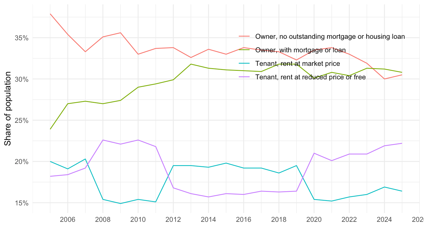

Housing Tenure Status

Javascript

Code

ilc_lvho02 |>
  filter(rskpovth %in% c("TOTAL"),
         hhcomp == "TOTAL",
         time == "2019",
         !(tenure %in% c("TOTAL"))) |>
  
  
  select(Tenure, Geo, values) |>
  spread(Tenure, values) %>%
  {if (is_html_output()) datatable(., filter = 'top', rownames = F) else .}

png

Code

include_graphics3b("bib/eurostat/ilc_lvho02_ex1-0.png")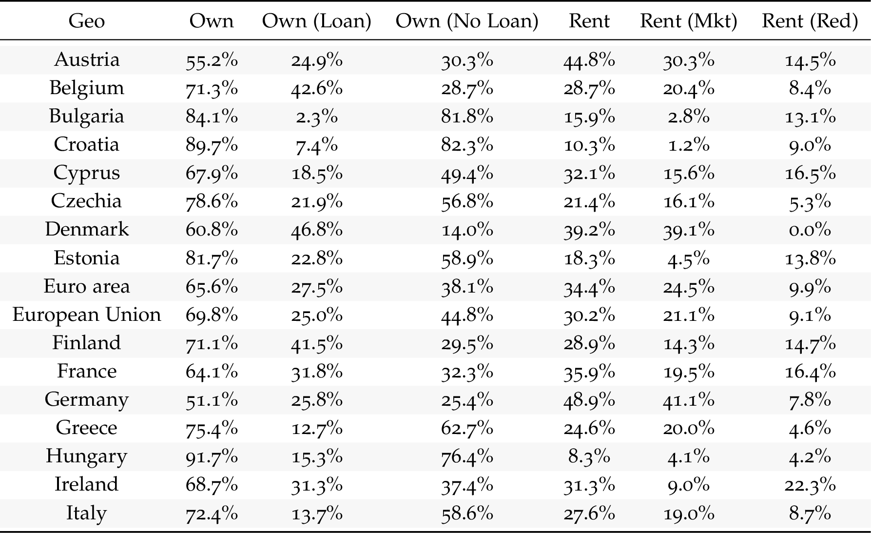

Code

include_graphics3b("bib/eurostat/ilc_lvho02_ex1-1.png")

Weights in HICP

Javascript

Code

data1 <- prc_hicp_inw |>
  filter(time %in% c("2019"),
         coicop == "CP041") |>
  transmute(geo, Geo, `Rent in HICP (%)` = round(values/10, 1))

data2 <- ilc_lvho02 |>
  filter(rskpovth == "TOTAL",
         hhcomp == "TOTAL",
         time == "2019",
         tenure == "RENT") |>
  transmute(geo, `Share of renters (%)` = values)


data1 |>
  inner_join(data2, by = "geo") |>
  
  mutate(Geo = ifelse(geo == "DE", "Germany", Geo)) |>
  select(1,4, 2, 3) %>%
  {if (is_html_output()) datatable(., filter = 'top', rownames = F) else .}

png

Code

include_graphics3b("bib/eurostat/ilc_lvho02_ex2.png")

AFGAP Graph

English

Association Française des Gestionnaires Actif-Passif - AFGAP. pdf

Code

data1 |>
  inner_join(data2, by = "geo") |>
  
  mutate(Geo = ifelse(geo == "DE", "Germany", Geo)) |>
  filter(!(geo %in% c("EA18", "EA", "EU", "EU27_2020", "EU28"))) |>
  ggplot() + theme_minimal() + xlab("Share of renters") + ylab("Rent share in HICP") +
  geom_point(aes(x = `Share of renters (%)`/100, y = `Rent in HICP (%)`/100)) +
  scale_x_continuous(breaks = 0.01*seq(-100, 100, 5),
                     labels = percent_format(accuracy = 1)) +
  scale_y_continuous(breaks = 0.01*seq(-100, 100, 2),
                     labels = percent_format(accuracy = 1)) +
  stat_smooth(aes(x = `Share of renters (%)`/100, y = `Rent in HICP (%)`/100), 
              linetype = 2, method = "lm", color = "#F2A900") +
  geom_text_repel(aes(x = `Share of renters (%)`/100, y = `Rent in HICP (%)`/100, label = Geo))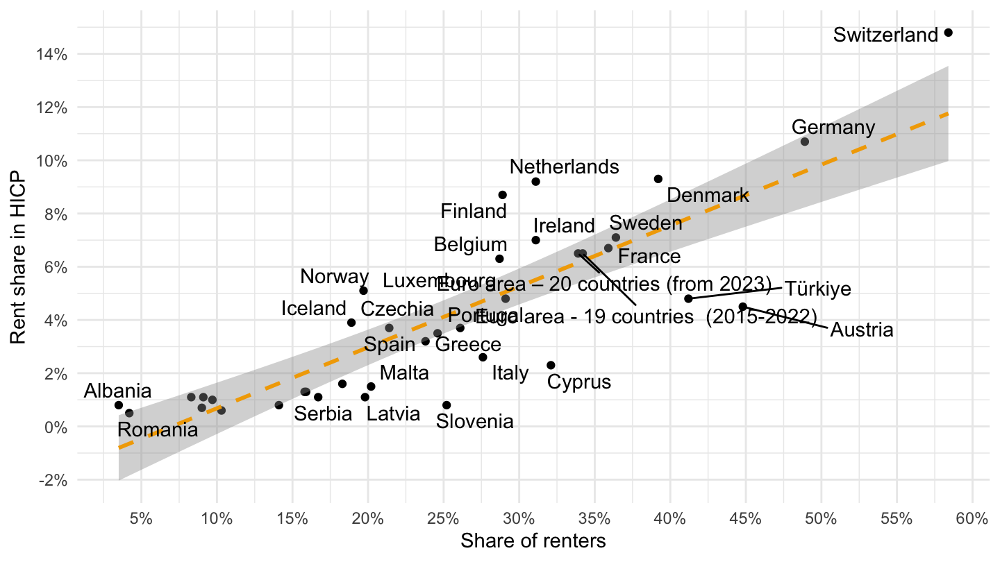

French

Code

geo <- read_parquet("geo_fr.parquet")
data1 |>
  inner_join(data2, by = "geo") |>
  
  mutate(Geo = ifelse(geo == "DE", "Germany", Geo)) |>
  filter(!(geo %in% c("EA18", "EA", "EU", "EU27_2020", "EU28"))) |>
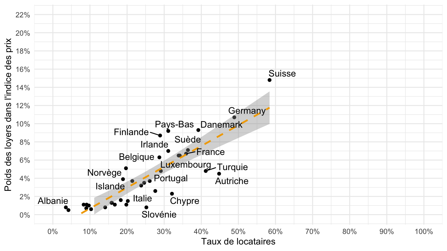
  ggplot() + theme_minimal() + xlab("Taux de locataires") + ylab("Poids des loyers dans l'indice des prix") +
  geom_point(aes(x = `Share of renters (%)`/100, y = `Rent in HICP (%)`/100)) +
  scale_x_continuous(breaks = 0.01*seq(-100, 100, 10),
                     labels = percent_format(accuracy = 1),
                     limits = c(0, 1)) +
  scale_y_continuous(breaks = 0.01*seq(-100, 100, 2),
                     labels = percent_format(accuracy = 1),
                     limits = c(0, 0.22)) +
  stat_smooth(aes(x = `Share of renters (%)`/100, y = `Rent in HICP (%)`/100), 
              linetype = 2, method = "lm", color = "#F2A900") +
  geom_text_repel(aes(x = `Share of renters (%)`/100, y = `Rent in HICP (%)`/100, label = Geo))