Distribution of income by different income groups - EU-SILC and ECHP surveys - ilc_di02

Data - Eurostat

Author

François Geerolf

Info

Last observation: Annual: 2025 (N = 1,316)

First observation: Annual: 1995 (N = 504)

Last data update: 23 jul 2026, 22:21. Last compile: 25 jul 2026, 20:14

Structure

Median Income Above 60% Threshold: France, Germany, Italy, Spain

Code

ilc_di02 %>%
  filter(geo %in% c("FR", "DE", "IT", "ES"),
         rskpovth == "A_60",
         unit == "EUR",
         statinfo == "MED_EI") %>%
  time_to_date %>%

  left_join(colors, by = c("Geo" = "country")) %>%
  mutate(values = values/1000) %>%
  ggplot + geom_line(aes(x = date, y = values, color = color)) +
  theme_minimal() + scale_color_identity() + add_4flags +
  scale_x_date(breaks = as.Date(paste0(seq(1990, 2100, 2), "-01-01")),
               labels = date_format("%Y")) +
  theme(legend.position = c(0.2, 0.85),
        legend.title = element_blank()) +
  xlab("") + ylab("Median income, above 60% threshold (thousand €)")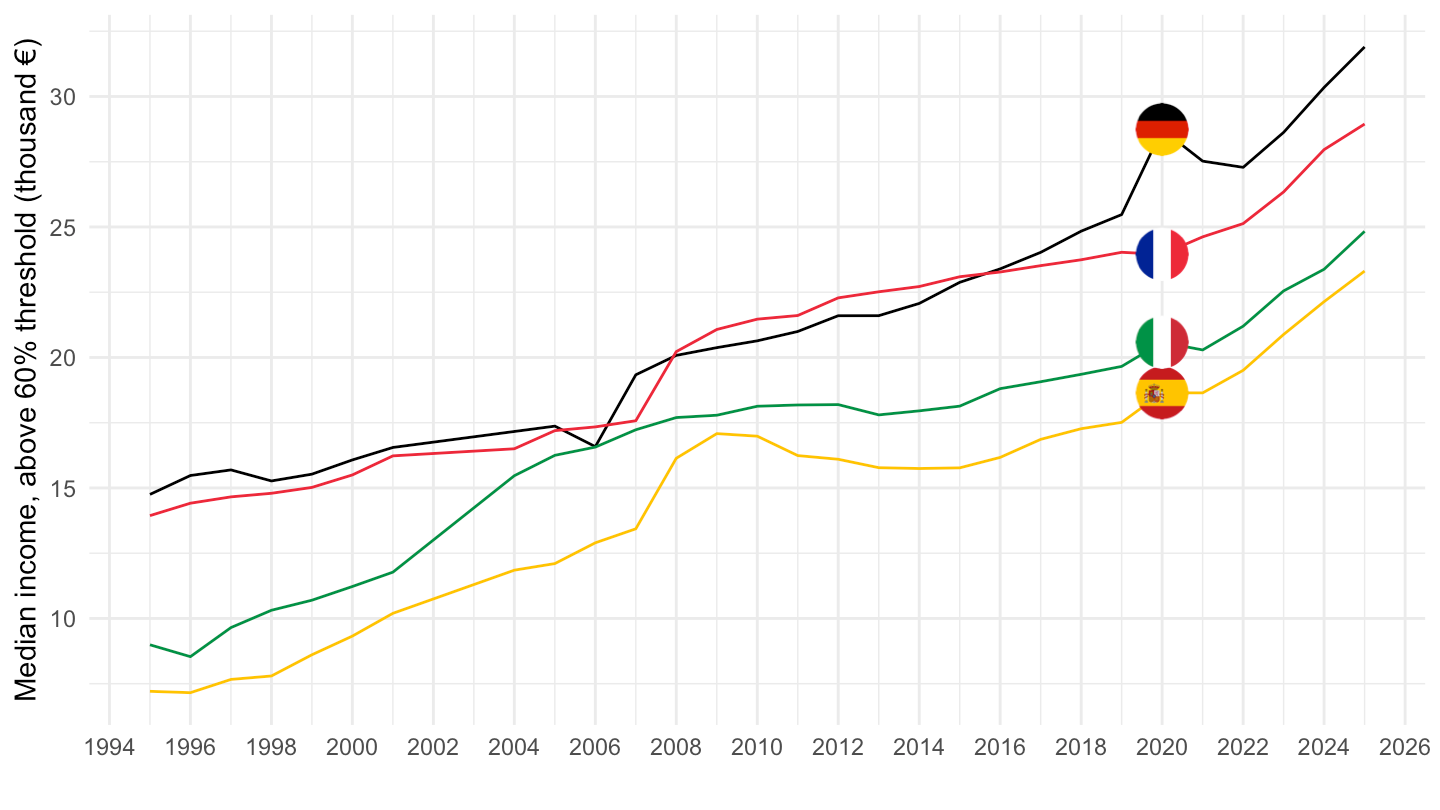

Above vs. Below 60% Threshold: France

Code

ilc_di02 %>%
  filter(geo == "FR",
         rskpovth %in% c("A_60", "B_60"),
         unit == "EUR",
         statinfo == "MED_EI") %>%
  time_to_date %>%

  mutate(values = values/1000) %>%
  ggplot + geom_line(aes(x = date, y = values, color = Rskpovth)) +
  theme_minimal() +
  scale_x_date(breaks = as.Date(paste0(seq(1990, 2100, 2), "-01-01")),
               labels = date_format("%Y")) +
  theme(legend.position = c(0.25, 0.85),
        legend.title = element_blank()) +
  xlab("") + ylab("Median equivalised income (thousand €)")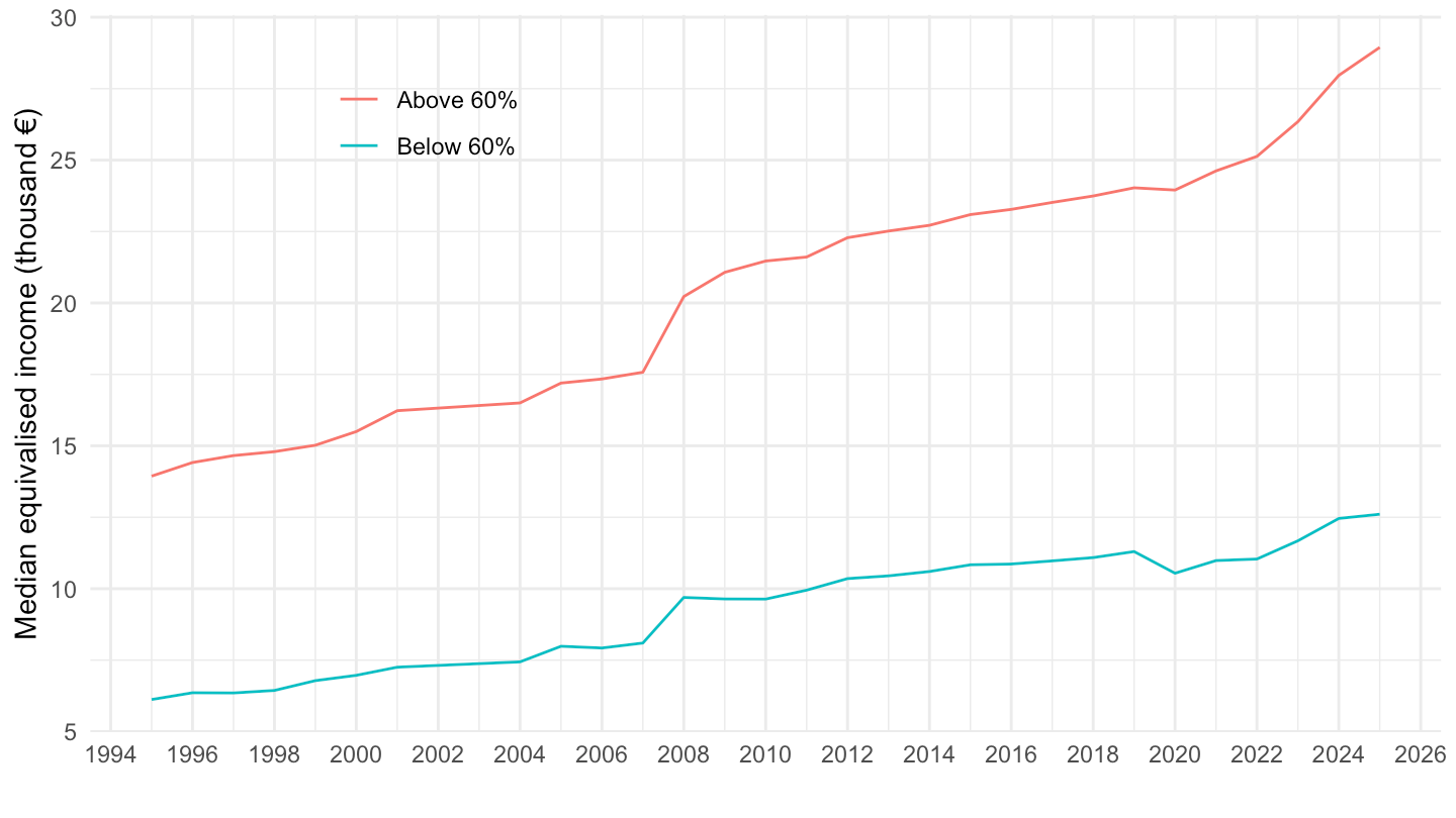

Latest Year by Country

Code

latest_y <- ilc_di02 %>%
  filter(rskpovth == "A_60",
         unit == "EUR",
         statinfo == "MED_EI",
         geo == "EU27_2020",
         !is.na(values)) %>%
  summarise(m = max(time)) %>%
  pull(m)

ilc_di02 %>%
  filter(rskpovth %in% c("A_60", "B_60"),
         unit == "EUR",
         statinfo == "MED_EI",
         geo %in% c("EU27_2020", "FR", "DE", "IT", "ES", "PT", "EL", "NL", "SE", "PL"),
         time == latest_y) %>%
  select(Geo, Rskpovth, values) %>%
  spread(Rskpovth, values) %>%
  arrange(-`Above 60%`) %>%
  print_table_conditional()

Geo	Above 60%	Below 60%
Netherlands	37172	17371
Germany	31900	13573
Sweden	31229	13192
France	28945	12607
European Union - 27 countries (from 2020)	25296	10576
Italy	24834	9982
Spain	23312	8938
Portugal	15872	6715
Poland	15373	6934
Greece	13153	5493

MD40 / MD70

Code

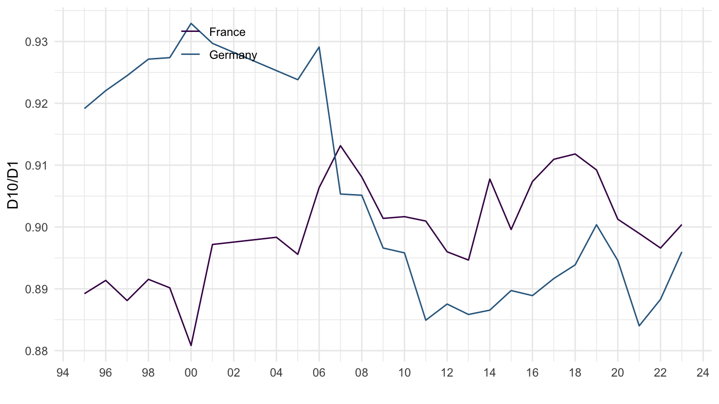
ilc_di02 %>%
  filter(rskpovth %in% c("A_40", "A_70"),
         geo %in% c("FR", "DE"),
         unit == "EUR",
         statinfo == "MED_EI") %>%
  time_to_date %>%

  arrange(date, rskpovth, geo, values) %>%
  spread(rskpovth, values) %>%
  mutate(D1D10 = A_40/A_70) %>%
  mutate(values = D1D10) %>%
  left_join(colors, by = c("Geo" = "country")) %>%
  ggplot() + geom_line(aes(x = date, y = values, color = color)) +
  scale_color_identity() + add_flags +
  theme_minimal() +
  scale_x_date(breaks = seq(1920, 2100, 2) %>% paste0("-01-01") %>% as.Date,
               labels = date_format("%Y")) +
  theme(legend.position = c(0.25, 0.9),
        legend.title = element_blank()) +
  scale_y_continuous(breaks = seq(0, 1, 0.01)) +
  ylab("D10/D1") + xlab("")