
Last observation: 2020 (N = 116)
First observation: 2010 (N = 106)
Last data update: 09 sept. 2026, 07:44
Last compile: 24 oct. 2026, 00:58
icw_sr_13 |>
  filter(geo %in% c("FR", "DE", "IT", "ES"),
         deg_urb == "TOTAL") |>
  year_to_date() |>
  add_flag_color("Geo") |>
  mutate(values = values/100) |>
  ggplot() + geom_line(aes(x = date, y = values, color = color)) +
  geom_point(aes(x = date, y = values, color = color)) +
  theme_minimal() + scale_color_identity() + add_flags +
  scale_x_date(breaks = as.Date(paste0(seq(2005, 2100, 5), "-01-01")),
               labels = date_format("%Y")) +
  xlab("") + ylab("Median saving rate (% of disposable income)") +
  scale_y_continuous(labels = scales::percent_format(accuracy = 1)) +
  geom_hline(yintercept = 0, linetype = "dashed", color = "black")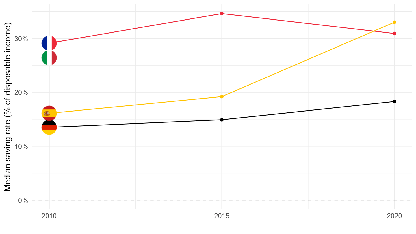
latest_y <- icw_sr_13 |>
  filter(geo %in% c("SE", "FR", "DE"),
         !is.na(values)) |>
  summarise(m = max(time)) |>
  pull(m)

icw_sr_13 |>
  filter(time == latest_y,
         geo %in% c("SE", "FR", "DE")) |>
  add_flag_color("Geo") |>
  ggplot() + geom_line(aes(x = deg_urb, y = values/100, color = color, group = Geo)) +
  scale_color_identity() + theme_minimal() +
  theme(legend.position = c(0.5, 0.7),
        legend.title = element_blank()) +
  xlab("by degree of urbanisation") + ylab("Median saving rate") +
  scale_y_continuous(breaks = 0.01*seq(-30, 50, 5),
                     labels = percent_format(accuracy = 1))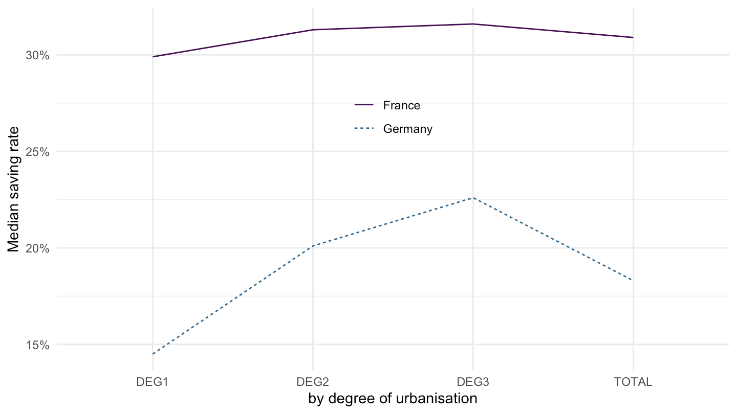
icw_sr_13 |>
  filter(time == latest_y) |>
  select(deg_urb, geo, Geo, values) |>
  spread(deg_urb, values) |>
  select(geo, Geo, everything()) %>%
{if (is_html_output()) print_table(.) else .}| geo | Geo | DEG1 | DEG2 | DEG3 | TOTAL |
|---|---|---|---|---|---|
| AT | Austria | 18.6 | 24.2 | 27.1 | 23.8 |
| BE | Belgium | 26.2 | 36.3 | 35.8 | 33.7 |
| BG | Bulgaria | 31.7 | 27.1 | 20.0 | 26.8 |
| CY | Cyprus | 25.7 | 24.0 | 24.4 | 25.1 |
| CZ | Czechia | 33.2 | 29.4 | 31.3 | 31.2 |
| DE | Germany | 14.5 | 20.1 | 22.6 | 18.3 |
| DK | Denmark | 30.8 | 39.2 | 36.1 | 35.0 |
| EA | Euro area (EA11-1999, EA12-2001, EA13-2007, EA15-2008, EA16-2009, EA17-2011, EA18-2014, EA19-2015, EA20-2023, EA21-2026) | 24.1 | 25.9 | 27.6 | 25.6 |
| EA21 | Euro area – 21 countries (from 2026) | 24.3 | 25.8 | 27.2 | 25.6 |
| EE | Estonia | 42.5 | 39.4 | 41.7 | 41.6 |
| EL | Greece | 14.5 | 16.1 | 16.5 | 15.6 |
| ES | Spain | 34.7 | 30.7 | 31.3 | 33.0 |
| EU | European Union (EU6-1958, EU9-1973, EU10-1981, EU12-1986, EU15-1995, EU25-2004, EU27-2007, EU28-2013, EU27-2020) | 25.9 | 27.0 | 27.2 | 26.6 |
| EU27_2020 | European Union - 27 countries (from 2020) | 25.9 | 27.0 | 27.2 | 26.6 |
| FI | Finland | 14.5 | 16.3 | 17.2 | 15.8 |
| FR | France | 29.9 | 31.3 | 31.6 | 30.9 |
| HR | Croatia | 22.0 | 20.5 | 17.5 | 19.8 |
| HU | Hungary | 21.9 | 20.6 | 20.8 | 21.1 |
| IE | Ireland | 31.4 | 33.6 | 24.4 | 29.2 |
| LT | Lithuania | 47.0 | 41.8 | 42.6 | 44.7 |
| LU | Luxembourg | 29.7 | 27.1 | 30.7 | 28.7 |
| LV | Latvia | 28.4 | 30.9 | 32.2 | 30.0 |
| MT | Malta | 27.7 | 31.2 | 25.7 | 29.4 |
| NL | Netherlands | 15.9 | 23.7 | 24.0 | 19.4 |
| PL | Poland | 49.8 | 51.0 | 50.1 | 50.2 |
| PT | Portugal | 34.7 | 33.2 | 30.6 | 33.3 |
| RO | Romania | 2.5 | 3.2 | -8.0 | -1.0 |
| SI | Slovenia | 22.3 | 22.8 | 23.1 | 22.8 |
| SK | Slovakia | 28.1 | 27.4 | 29.0 | 28.2 |
icw_sr_13 |>
  filter(time == "2010") |>
  select(deg_urb, geo, Geo, values) |>

  spread(deg_urb, values) |>
  select(geo, Geo, everything()) %>%
{if (is_html_output()) print_table(.) else .}| geo | Geo | DEG1 | DEG2 | DEG3 | TOTAL |
|---|---|---|---|---|---|
| AT | Austria | 14.6 | 21.4 | 19.7 | 18.0 |
| BE | Belgium | 7.2 | 11.5 | 6.6 | 8.9 |
| BG | Bulgaria | 43.4 | 40.1 | 31.5 | 38.0 |
| CY | Cyprus | 13.8 | 6.1 | 11.5 | 12.2 |
| CZ | Czechia | 23.1 | 25.1 | 23.9 | 23.9 |
| DE | Germany | 12.6 | 15.2 | 12.2 | 13.5 |
| DK | Denmark | 1.5 | 5.3 | 6.7 | 4.3 |
| EE | Estonia | 37.0 | 36.0 | 32.7 | 34.9 |
| EL | Greece | -12.5 | -9.2 | -10.8 | -11.2 |
| ES | Spain | 19.8 | 13.0 | 11.3 | 16.1 |
| FI | Finland | 21.6 | 21.7 | 23.1 | 22.2 |
| FR | France | 28.9 | 29.8 | 28.0 | 29.1 |
| HR | Croatia | 10.1 | 7.2 | -3.7 | 4.0 |
| HU | Hungary | 17.2 | 15.3 | 16.1 | 16.3 |
| IE | Ireland | 21.4 | 16.8 | 16.7 | 18.4 |
| IT | Italy | 29.0 | 25.5 | 21.7 | 26.4 |
| LT | Lithuania | 31.2 | NA | 16.3 | 22.8 |
| LU | Luxembourg | 24.7 | 27.6 | 37.8 | 28.4 |
| LV | Latvia | 12.1 | 17.2 | 8.6 | 10.5 |
| MT | Malta | 13.6 | 14.0 | NA | 13.7 |
| PL | Poland | 26.4 | 25.4 | 22.4 | 24.7 |
| PT | Portugal | 14.8 | 9.1 | 15.1 | 13.1 |
| RO | Romania | 3.7 | -0.9 | -11.5 | -5.1 |
| SE | Sweden | 14.6 | 23.1 | 18.3 | 18.0 |
| SI | Slovenia | 18.9 | 18.6 | 17.1 | 18.0 |
| SK | Slovakia | 28.2 | 22.2 | 23.7 | 24.4 |
| UK | United Kingdom | 22.3 | 23.7 | 23.8 | 22.9 |
icw_sr_13 |>
  filter(time == "2015") |>
  select(deg_urb, geo, Geo, values) |>

  spread(deg_urb, values) |>
  select(geo, Geo, everything()) %>%
{if (is_html_output()) print_table(.) else .}| geo | Geo | DEG1 | DEG2 | DEG3 | TOTAL |
|---|---|---|---|---|---|
| AT | Austria | 16.8 | 21.6 | 24.5 | 21.1 |
| BE | Belgium | 16.5 | 20.1 | 20.1 | 19.0 |
| BG | Bulgaria | 19.7 | 16.1 | 14.2 | 17.4 |
| CY | Cyprus | 9.9 | 11.0 | 10.8 | 10.5 |
| CZ | Czechia | 25.0 | 25.2 | 26.2 | 25.5 |
| DE | Germany | 11.0 | 16.6 | 19.5 | 14.9 |
| DK | Denmark | 17.8 | 28.4 | 30.9 | 25.6 |
| EA | Euro area (EA11-1999, EA12-2001, EA13-2007, EA15-2008, EA16-2009, EA17-2011, EA18-2014, EA19-2015, EA20-2023, EA21-2026) | 19.7 | 20.0 | 23.3 | 20.7 |
| EA21 | Euro area – 21 countries (from 2026) | 19.7 | 19.7 | 22.6 | 20.5 |
| EE | Estonia | 37.3 | 31.8 | 33.2 | 34.9 |
| EL | Greece | -4.8 | -6.0 | -8.8 | -6.5 |
| ES | Spain | 21.3 | 18.9 | 15.7 | 19.2 |
| EU | European Union (EU6-1958, EU9-1973, EU10-1981, EU12-1986, EU15-1995, EU25-2004, EU27-2007, EU28-2013, EU27-2020) | 19.0 | 19.8 | 22.0 | 20.1 |
| EU27_2020 | European Union - 27 countries (from 2020) | 20.4 | 20.5 | 22.2 | 21.0 |
| FI | Finland | 17.9 | 19.5 | 21.7 | 19.5 |
| FR | France | 33.3 | 34.9 | 36.3 | 34.6 |
| HR | Croatia | 10.6 | 5.5 | -0.3 | 4.4 |
| HU | Hungary | 15.1 | 13.4 | 14.8 | 14.6 |
| IE | Ireland | 27.1 | 24.2 | 24.1 | 25.2 |
| LT | Lithuania | 37.7 | 23.4 | 26.0 | 31.6 |
| LU | Luxembourg | 25.3 | 23.7 | 30.4 | 27.0 |
| LV | Latvia | 25.7 | 23.5 | 23.7 | 24.6 |
| MT | Malta | 17.7 | 19.2 | NA | 17.8 |
| NL | Netherlands | 12.9 | 19.2 | 19.5 | 15.8 |
| PL | Poland | 30.9 | 30.1 | 27.4 | 29.5 |
| PT | Portugal | 19.7 | 18.5 | 17.8 | 18.9 |
| RO | Romania | 12.3 | 11.3 | 9.6 | 10.9 |
| SE | Sweden | 23.9 | 25.2 | 24.8 | 24.6 |
| SI | Slovenia | 23.4 | 23.7 | 22.2 | 22.8 |
| SK | Slovakia | 18.6 | 17.6 | 16.9 | 17.6 |
| UK | United Kingdom | 13.4 | 15.2 | 20.0 | 15.0 |
icw_sr_13 |>
  filter(time == "2015",
         geo %in% c("SE", "FR", "DE")) |>

  add_flag_color("Geo") |>
  ggplot() + geom_line(aes(x = deg_urb, y = values/100, color = color, group = Geo)) +
  scale_color_identity() + theme_minimal() +
  theme(legend.position = c(0.5, 0.7),
        legend.title = element_blank()) +
  xlab("by degree of urbanisation") + ylab("Median saving rate") +
  scale_y_continuous(breaks = 0.01*seq(-30, 50, 5),
                     labels = percent_format(accuracy = 1))