Aggregate propensity to consume by income quintile - experimental statistics - icw_sr_10

Data - Eurostat

Info

Last observation: Annual: 2020 (N = 174)

First observation: Annual: 2010 (N = 158)

Last data update: 23 jul 2026, 22:25. Last compile: 24 jul 2026, 02:00

Structure

freq

quant_inc

unit

geo

Propensity to Consume by Income Quintile: France

icw_sr_10 %>%
  filter(geo == "FR",
         quant_inc %in% c("QU1", "QU3", "QU5", "TOTAL")) %>%
  year_to_date %>%
  mutate(values = values/100) %>%
  ggplot + geom_line(aes(x = date, y = values, color = Quant_inc)) +
  theme_minimal() +
  scale_x_date(breaks = as.Date(paste0(seq(2010, 2100, 5), "-01-01")),
               labels = date_format("%Y")) +
  theme(legend.position = c(0.75, 0.85),
        legend.title = element_blank()) +
  xlab("") + ylab("Consumption expenditure, % of disposable income") +
  scale_y_continuous(labels = scales::percent_format(accuracy = 1)) +
  geom_hline(yintercept = 1, linetype = "dashed", color = "black")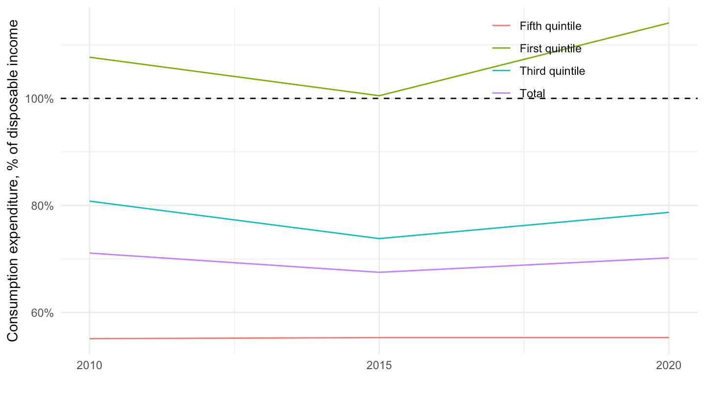

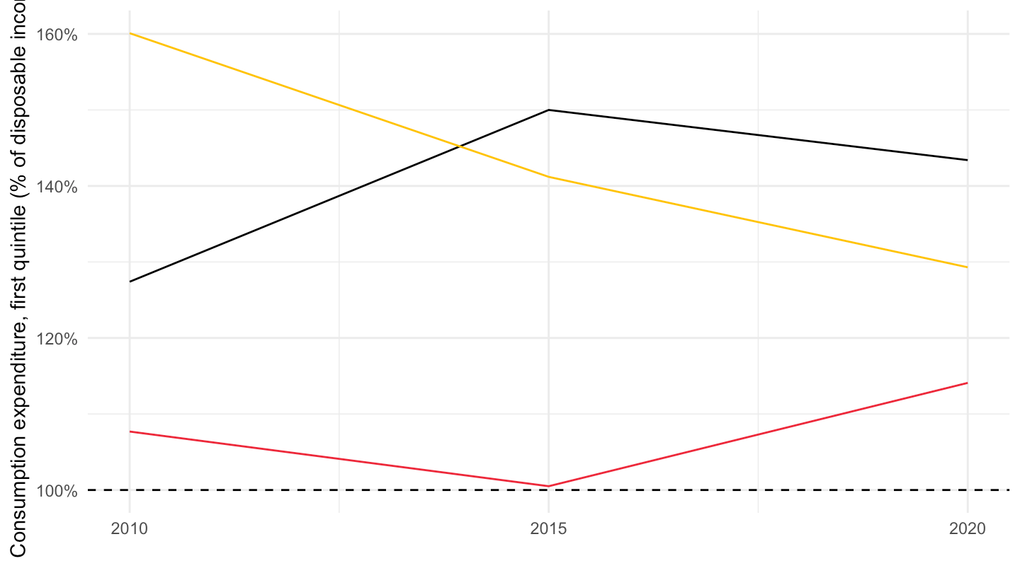
Bottom Income Quintile: France, Germany, Italy, Spain

icw_sr_10 %>%
  filter(geo %in% c("FR", "DE", "IT", "ES"),
         quant_inc == "QU1") %>%
  year_to_date %>%
  left_join(colors, by = c("Geo" = "country")) %>%
  mutate(values = values/100) %>%
  ggplot + geom_line(aes(x = date, y = values, color = color)) +
  theme_minimal() + scale_color_identity() + add_4flags +
  scale_x_date(breaks = as.Date(paste0(seq(2010, 2100, 5), "-01-01")),
               labels = date_format("%Y")) +
  theme(legend.position = c(0.25, 0.2),
        legend.title = element_blank()) +
  xlab("") + ylab("Consumption expenditure, first quintile (% of disposable income)") +
  scale_y_continuous(labels = scales::percent_format(accuracy = 1)) +
  geom_hline(yintercept = 1, linetype = "dashed", color = "black")