Business enterprise R&D personnel in high-tech sectors - NACE Rev. 2 - htec_sti_pers2

Data - Eurostat

Info

Last observation: 2024 (N = 148)

First observation: 2005 (N = 260)

Last data update: 14 aoû 2026, 19:23. Last compile: 18 aoû 2026, 01:25

Structure

freq

nace_r2

unit

prof_pos

geo

R&D Researchers in High-Tech Manufacturing

France, Germany, Italy, Spain, Poland

htec_sti_pers2 |>
  filter(geo %in% c("FR", "DE", "IT", "ES", "PL"),
         nace_r2 == "C_HTC",
         unit == "HC",
         prof_pos == "RSE") |>
  year_to_date() |>
  left_join(colors, by = c("Geo" = "country")) |>
  ggplot() + geom_line(aes(x = date, y = values, color = color)) +
  theme_minimal() + scale_color_identity() + add_flags +
  scale_x_date(breaks = as.Date(paste0(seq(2000, 2100, 2), "-01-01")),
               labels = date_format("%Y")) +
  xlab("") + ylab("R&D researchers, high-tech manufacturing (head count)")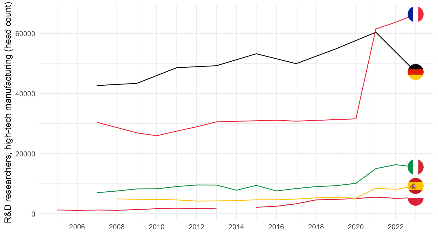

France: High-Tech vs. Low-Tech Manufacturing

htec_sti_pers2 |>
  filter(geo == "FR",
         nace_r2 %in% c("C_HTC", "C_HTC_M", "C_LTC", "C_LTC_M"),
         unit == "HC",
         prof_pos == "RSE") |>
  year_to_date() |>
  ggplot() + geom_line(aes(x = date, y = values, color = Nace_r2)) +
  theme_minimal() +
  scale_x_date(breaks = as.Date(paste0(seq(2000, 2100, 2), "-01-01")),
               labels = date_format("%Y")) +
  xlab("") + ylab("R&D researchers (head count)")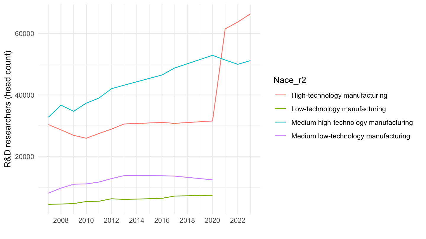

Latest Year by Country

latest_y <- htec_sti_pers2 |>
  filter(geo %in% c("FR", "DE", "IT", "ES", "PL", "NL", "BE", "SE"),
         nace_r2 %in% c("C_HTC", "C"),
         unit == "HC",
         prof_pos == "RSE",
         !is.na(values)) |>
  summarise(m = max(time)) |>
  pull(m)

htec_sti_pers2 |>
  filter(geo %in% c("FR", "DE", "IT", "ES", "PL", "NL", "BE", "SE"),
         nace_r2 %in% c("C_HTC", "C"),
         unit == "HC",
         prof_pos == "RSE",
         time == latest_y) |>
  select(Geo, Nace_r2, values) |>
  spread(Nace_r2, values) |>
  arrange(-`High-technology manufacturing`) |>
  print_table_conditional()

Geo	High-technology manufacturing	Manufacturing
France	66357	135378
Germany	47147	252550
Italy	15529	NA
Spain	9238	27636
Belgium	7920	NA
Poland	5325	36575
Netherlands	NA	NA
Sweden	NA	46451