Mean consumption expenditure by income quintile - hbs_exp_t133

Data - Eurostat

Author

François Geerolf

Info

Last observation: Annual: 2020 (N = 348)

First observation: Annual: 1988 (N = 120)

Last data update: 23 jul 2026, 22:08. Last compile: 24 jul 2026, 01:47

Structure

Household Consumption Expenditure

France, Germany, Italy, Spain

Code

hbs_exp_t133 %>%
  filter(geo %in% c("FR", "DE", "IT", "ES"),
         quant_inc == "TOTAL",
         unit == "PPS_AE") %>%
  year_to_date %>%
  left_join(colors, by = c("Geo" = "country")) %>%
  mutate(color = ifelse(geo == "ES", color2, color)) %>%
  ggplot + geom_line(aes(x = date, y = values, color = color)) +
  geom_point(aes(x = date, y = values, color = color)) +
  theme_minimal() + scale_color_identity() + add_4flags +
  scale_x_date(breaks = as.Date(paste0(seq(1985, 2100, 5), "-01-01")),
               labels = date_format("%Y")) +
  xlab("") + ylab("Mean consumption expenditure (PPS per adult equivalent)")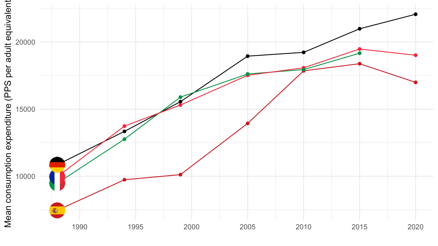

Quintile Ratio (Q5/Q1): France, Germany, Spain

Code

hbs_exp_t133 %>%
  filter(geo %in% c("FR", "DE", "ES"),
         quant_inc %in% c("QU1", "QU5"),
         unit == "PPS_AE") %>%
  select(geo, Geo, quant_inc, time, values) %>%
  spread(quant_inc, values) %>%
  mutate(values = QU5 / QU1) %>%
  year_to_date %>%
  left_join(colors, by = c("Geo" = "country")) %>%
  ggplot + geom_line(aes(x = date, y = values, color = color)) +
  geom_point(aes(x = date, y = values, color = color)) +
  theme_minimal() + scale_color_identity() + add_3flags +
  scale_x_date(breaks = as.Date(paste0(seq(1985, 2100, 5), "-01-01")),
               labels = date_format("%Y")) +
  xlab("") + ylab("Top vs. bottom quintile expenditure ratio (Q5 / Q1)")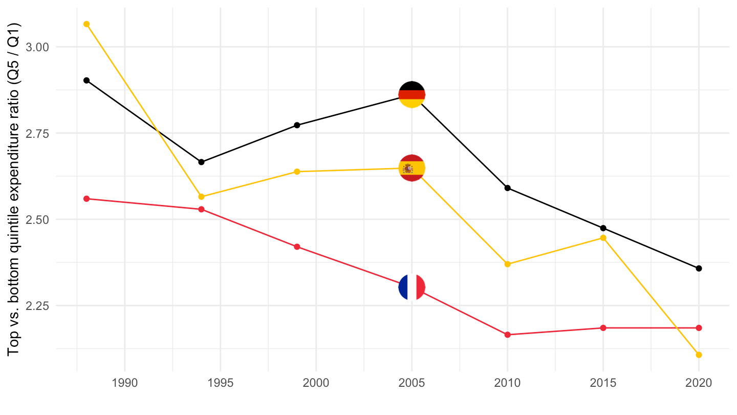

Latest Wave by Quintile

Code

latest_t <- hbs_exp_t133 %>%
  filter(geo %in% c("FR", "DE", "IT", "ES"), unit == "PPS_AE", !is.na(values)) %>%
  summarise(m = max(time)) %>%
  pull(m)

hbs_exp_t133 %>%
  filter(geo %in% c("FR", "DE", "IT", "ES"),
         unit == "PPS_AE",
         quant_inc %in% c("QU1", "QU2", "QU3", "QU4", "QU5"),
         time == latest_t) %>%
  select(Quant_inc, Geo, values) %>%
  spread(Geo, values) %>%
  print_table_conditional()

Quant_inc	France	Germany	Spain
Fifth quintile	27642	31368	23524
First quintile	12650	13305	11165
Fourth quintile	20792	25030	18553
Second quintile	15867	18504	14824
Third quintile	18151	22162	16928

2015

France, Germany, Italy

Code

hbs_exp_t133 %>%
  filter(time == "2015") %>%
  select_if(~ n_distinct(.) > 1) %>%
  spread(quant_inc, values)

# # A tibble: 414 × 12
#    Quant_inc   unit  Unit  geo   Geo     QU1   QU2   QU3   QU4   QU5 TOTAL   UNK
#    <chr>       <chr> <chr> <chr> <chr> <dbl> <dbl> <dbl> <dbl> <dbl> <dbl> <dbl>
#  1 Fifth quin… PPS_… Purc… AT    Aust…    NA    NA    NA    NA 28874    NA    NA
#  2 Fifth quin… PPS_… Purc… BE    Belg…    NA    NA    NA    NA 27496    NA    NA
#  3 Fifth quin… PPS_… Purc… BG    Bulg…    NA    NA    NA    NA 11717    NA    NA
#  4 Fifth quin… PPS_… Purc… CY    Cypr…    NA    NA    NA    NA 29926    NA    NA
#  5 Fifth quin… PPS_… Purc… CZ    Czec…    NA    NA    NA    NA 12374    NA    NA
#  6 Fifth quin… PPS_… Purc… DE    Germ…    NA    NA    NA    NA 30692    NA    NA
#  7 Fifth quin… PPS_… Purc… DK    Denm…    NA    NA    NA    NA 26885    NA    NA
#  8 Fifth quin… PPS_… Purc… EE    Esto…    NA    NA    NA    NA 18111    NA    NA
#  9 Fifth quin… PPS_… Purc… EL    Gree…    NA    NA    NA    NA 21713    NA    NA
# 10 Fifth quin… PPS_… Purc… ES    Spain    NA    NA    NA    NA 27049    NA    NA
# # ℹ 404 more rows