
Last observation: sept. 2026 (N = 20726)
First observation: janv. 2002 (N = 12107)
Last data update: 14 nov. 2026, 22:29
Last compile: 14 nov. 2026, 22:47
ext_st_eu27_2020sitc |>
  filter(stk_flow == "BAL_RT",
         indic_et == "TRD_VAL",
         sitc06 == "TOTAL",
         partner %in% c("US", "CN_X_HK", "UK", "JP")) |>
  month_to_date() |>
  mutate(values = values/1000) |>
  ggplot() + geom_line(aes(x = date, y = values, color = Partner)) +
  theme_minimal() +
  scale_x_date(breaks = as.Date(paste0(seq(2002, 2100, 2), "-01-01")),
               labels = date_format("%Y")) +
  theme(legend.position = c(0.2, 0.2),
        legend.title = element_blank()) +
  xlab("") + ylab("EU27 trade balance (Bn€)") +
  geom_hline(yintercept = 0, linetype = "dashed", color = "black")
Partner “CN_X_HK” is China excluding Hong Kong. Flows are in current euros; annual figures are sums of the 12 months of each calendar year, and the annual ratios to GDP use the annual current-price GDP of the EU27 (nama_10_gdp), and the quarterly ones the seasonally adjusted quarterly GDP (namq_10_gdp).
cn_tot <- annual_trade("CN_X_HK")

cn_tot |>
  mutate(values = values / 1000,
         flow = recode(stk_flow, EXP = "Exports to China", IMP = "Imports from China")) |>
  ggplot() + geom_col(aes(x = year, y = values, fill = flow), position = "dodge") +
  theme_minimal() +
  scale_x_continuous(breaks = seq(2002, 2100, 2)) +
  theme(legend.position = c(0.2, 0.8), legend.title = element_blank()) +
  xlab("") + ylab("EU27 trade with China (Bn€)")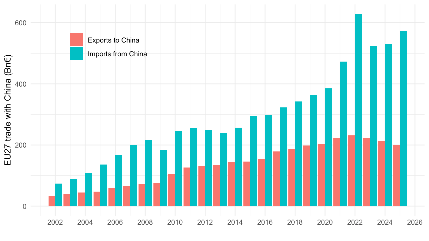
cn_tot |>
  select(year, stk_flow, values) |>
  pivot_wider(names_from = stk_flow, values_from = values) |>
  mutate(bal = (EXP - IMP) / 1000) |>
  ggplot() + geom_col(aes(x = year, y = bal), fill = "#C8102E") +
  theme_minimal() +
  scale_x_continuous(breaks = seq(2002, 2100, 2)) +
  xlab("") + ylab("EU27 trade balance with China (Bn€)")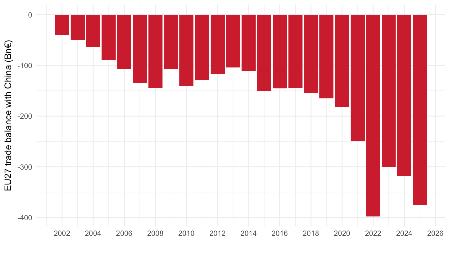
cn_tot |>
  mutate(flow = recode(stk_flow, EXP = "Exports to China", IMP = "Imports from China")) |>
  ggplot() + geom_line(aes(x = year, y = pct_gdp, color = flow), linewidth = 1) +
  geom_point(aes(x = year, y = pct_gdp, color = flow)) +
  theme_minimal() +
  scale_x_continuous(breaks = seq(2002, 2100, 2)) +
  scale_y_continuous(labels = scales::percent_format(scale = 1, accuracy = 0.1)) +
  theme(legend.position = c(0.2, 0.8), legend.title = element_blank()) +
  xlab("") + ylab("EU27 trade with China (% of EU27 GDP)")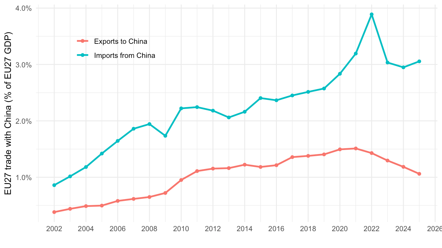
cn_tot |>
  select(year, stk_flow, pct_gdp) |>
  pivot_wider(names_from = stk_flow, values_from = pct_gdp) |>
  mutate(bal = EXP - IMP) |>
  ggplot() + geom_col(aes(x = year, y = bal), fill = "#C8102E") +
  theme_minimal() +
  scale_x_continuous(breaks = seq(2002, 2100, 2)) +
  scale_y_continuous(labels = scales::percent_format(scale = 1, accuracy = 0.1)) +
  xlab("") + ylab("EU27 trade balance with China (% of EU27 GDP)")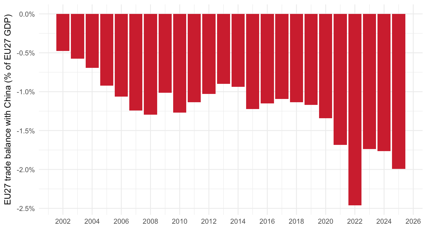
last_year <- max(cn_tot$year)

cn_tot |>
  filter(year %in% c(2002, last_year)) |>
  mutate(flow = recode(stk_flow, EXP = "Exports", IMP = "Imports"),
         year = factor(year)) |>
  ggplot(aes(x = flow, y = pct_gdp, fill = year)) +
  geom_col(position = "dodge") +
  geom_text(aes(label = sprintf("%.1f%%", pct_gdp)),
            position = position_dodge(width = 0.9), vjust = -0.4) +
  theme_minimal() +
  scale_fill_manual(values = c("#7A7A7A", "#C8102E")) +
  scale_y_continuous(labels = scales::percent_format(scale = 1, accuracy = 0.1),
                     expand = expansion(mult = c(0, 0.1))) +
  theme(legend.position = c(0.15, 0.85), legend.title = element_blank()) +
  xlab("") + ylab("EU27 trade with China (% of EU27 GDP)")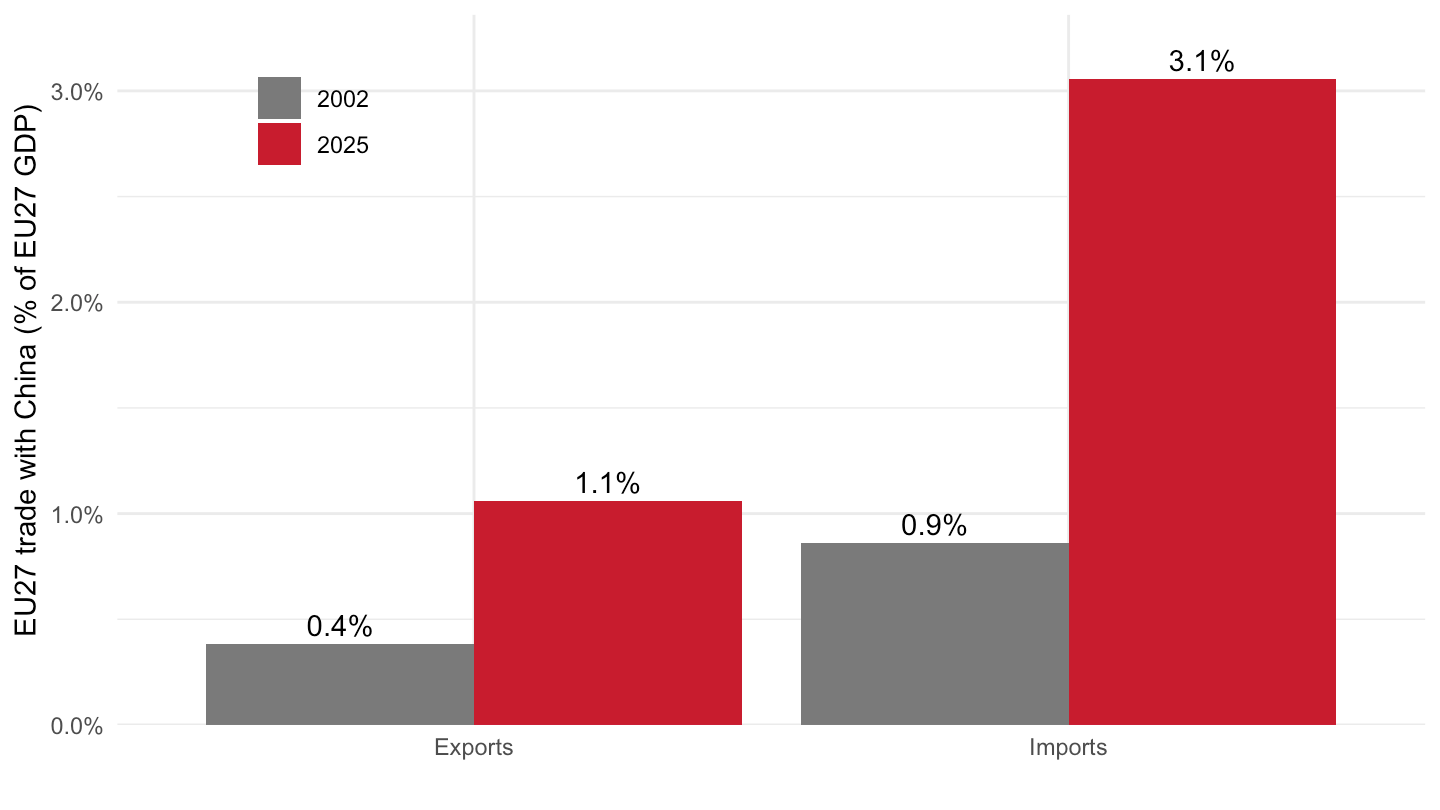
sitc_main <- c("SITC0", "SITC1", "SITC2", "SITC3", "SITC4", "SITC5", "SITC6", "SITC7", "SITC8")

cn_sitc <- annual_trade("CN_X_HK", sitc_main)

cn_sitc |>
  filter(year %in% c(2002, last_year)) |>
  select(year, sitc06, Sitc06, stk_flow, pct_gdp) |>
  pivot_wider(names_from = stk_flow, values_from = pct_gdp) |>
  mutate(bal = EXP - IMP,
         year = factor(year),
         Sitc06 = str_wrap(paste0(sitc06, " - ", Sitc06), 28)) |>
  ggplot(aes(x = bal, y = reorder(Sitc06, bal), fill = year)) +
  geom_col(position = "dodge") +
  theme_minimal() +
  scale_fill_manual(values = c("#7A7A7A", "#C8102E")) +
  scale_x_continuous(labels = scales::percent_format(scale = 1, accuracy = 0.1)) +
  theme(legend.position = "bottom", legend.title = element_blank()) +
  xlab("EU27 trade balance with China (% of EU27 GDP)") + ylab("")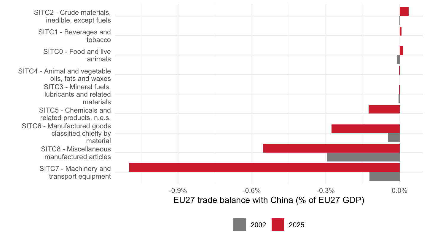
cn_sitc |>
  filter(stk_flow == "IMP") |>
  mutate(values = values / 1000,
         Sitc06 = paste0(sitc06, " - ", str_trunc(Sitc06, 30))) |>
  ggplot() + geom_area(aes(x = year, y = values, fill = Sitc06)) +
  theme_minimal() +
  scale_x_continuous(breaks = seq(2002, 2100, 2)) +
  theme(legend.position = "right", legend.title = element_blank()) +
  xlab("") + ylab("EU27 imports from China (Bn€)")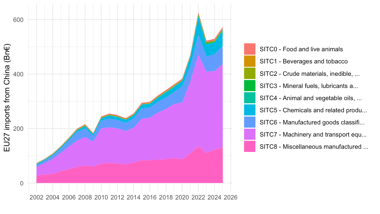
cn_sitc |>
  filter(stk_flow == "IMP") |>
  mutate(Sitc06 = paste0(sitc06, " - ", str_trunc(Sitc06, 30))) |>
  ggplot() + geom_area(aes(x = year, y = pct_gdp, fill = Sitc06)) +
  theme_minimal() +
  scale_x_continuous(breaks = seq(2002, 2100, 2)) +
  scale_y_continuous(labels = scales::percent_format(scale = 1, accuracy = 0.1)) +
  theme(legend.position = "right", legend.title = element_blank()) +
  xlab("") + ylab("EU27 imports from China (% of EU27 GDP)")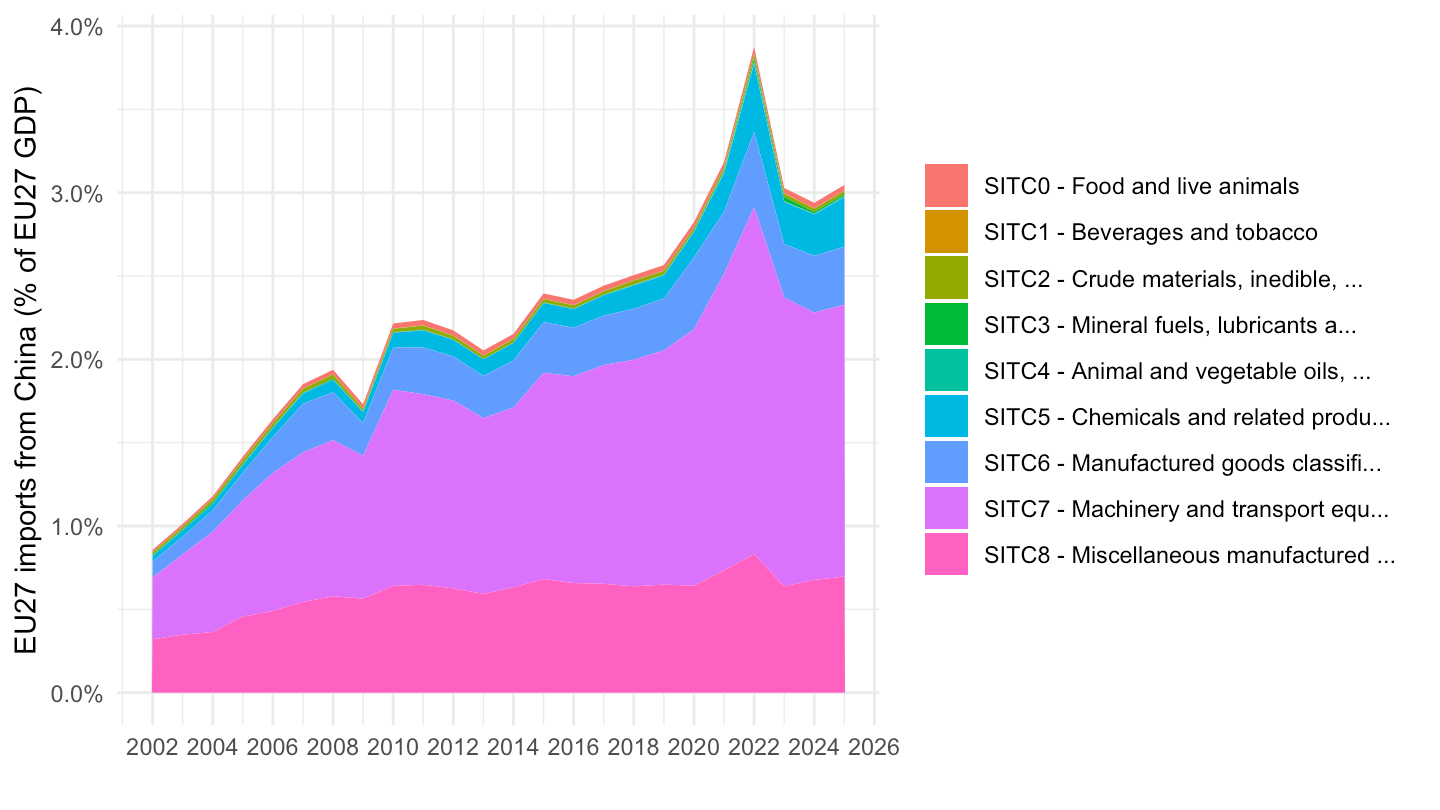
cn_sitc |>
  filter(stk_flow == "EXP", sitc06 %in% c("SITC7", "SITC5", "SITC6", "SITC8", "SITC3", "SITC0")) |>
  mutate(Sitc06 = paste0(sitc06, " - ", str_trunc(Sitc06, 30))) |>
  ggplot() + geom_line(aes(x = year, y = pct_gdp, color = Sitc06), linewidth = 1) +
  theme_minimal() +
  scale_x_continuous(breaks = seq(2002, 2100, 2)) +
  scale_y_continuous(labels = scales::percent_format(scale = 1, accuracy = 0.1)) +
  theme(legend.position = "right", legend.title = element_blank()) +
  xlab("") + ylab("EU27 exports to China (% of EU27 GDP)")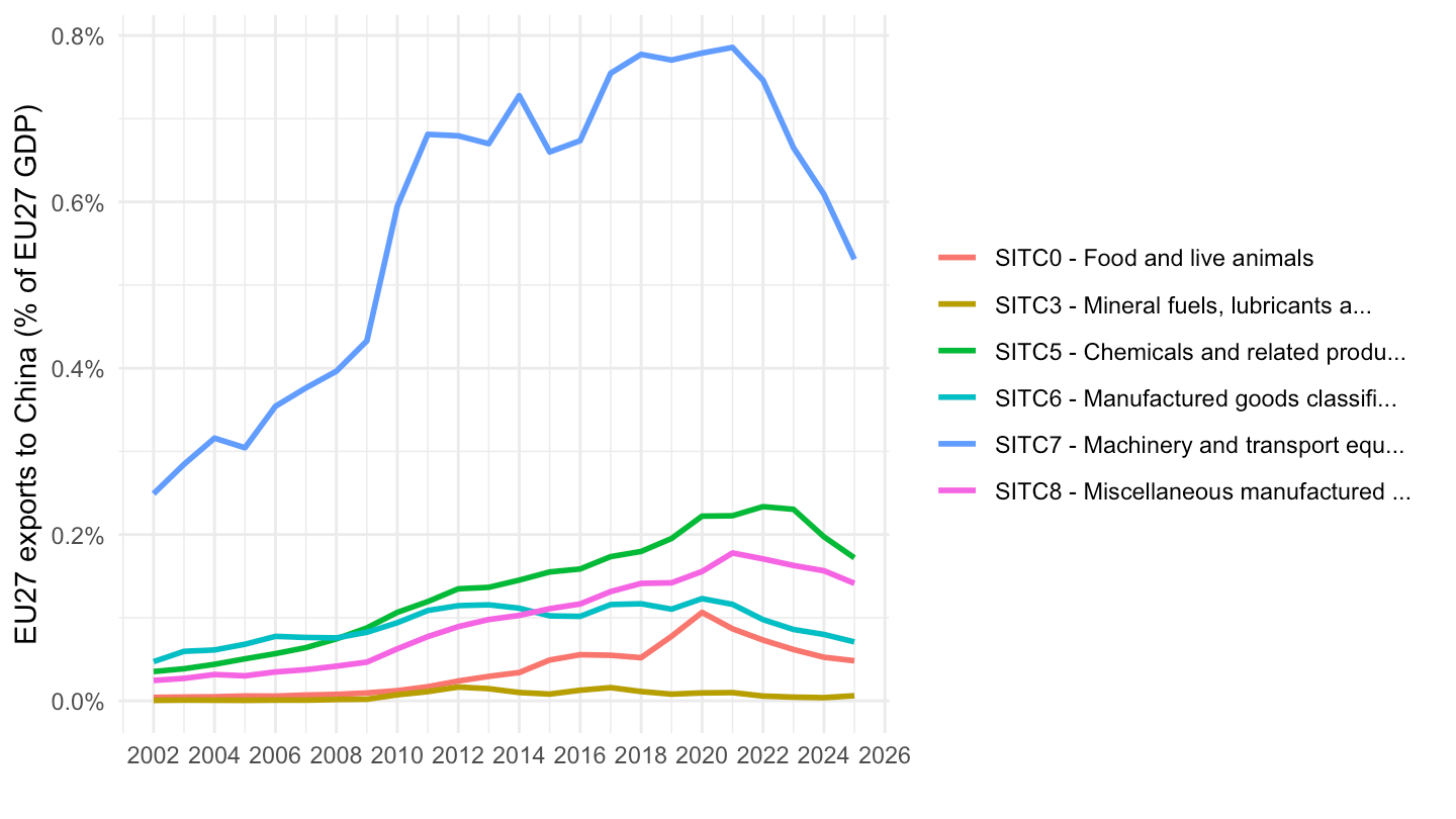
Quarterly trade is the sum of the three monthly values; both trade and GDP are then summed over the last four quarters, so that the ratio is not affected by seasonality and runs up to the latest quarter for which GDP is available.
cn_q <- quarterly_trade("CN_X_HK")

cn_q |>
  mutate(flow = recode(stk_flow, EXP = "Exports to China", IMP = "Imports from China")) |>
  ggplot() + geom_line(aes(x = date, y = pct_gdp, color = flow), linewidth = 1) +
  theme_minimal() +
  scale_x_date(breaks = as.Date(paste0(seq(2002, 2100, 2), "-01-01")),
               labels = date_format("%Y")) +
  scale_y_continuous(labels = scales::percent_format(scale = 1, accuracy = 0.1)) +
  theme(legend.position = c(0.2, 0.8), legend.title = element_blank()) +
  xlab("") + ylab("EU27 trade with China (% of EU27 GDP, 4Q sums)")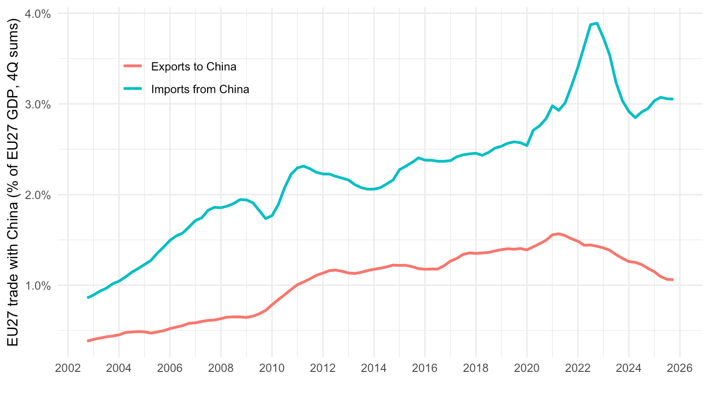
cn_q |>
  select(date, stk_flow, pct_gdp) |>
  pivot_wider(names_from = stk_flow, values_from = pct_gdp) |>
  mutate(bal = EXP - IMP) |>
  ggplot() + geom_line(aes(x = date, y = bal), color = "#C8102E", linewidth = 1) +
  theme_minimal() +
  scale_x_date(breaks = as.Date(paste0(seq(2002, 2100, 2), "-01-01")),
               labels = date_format("%Y")) +
  scale_y_continuous(labels = scales::percent_format(scale = 1, accuracy = 0.1)) +
  xlab("") + ylab("EU27 trade balance with China (% of EU27 GDP, 4Q sums)")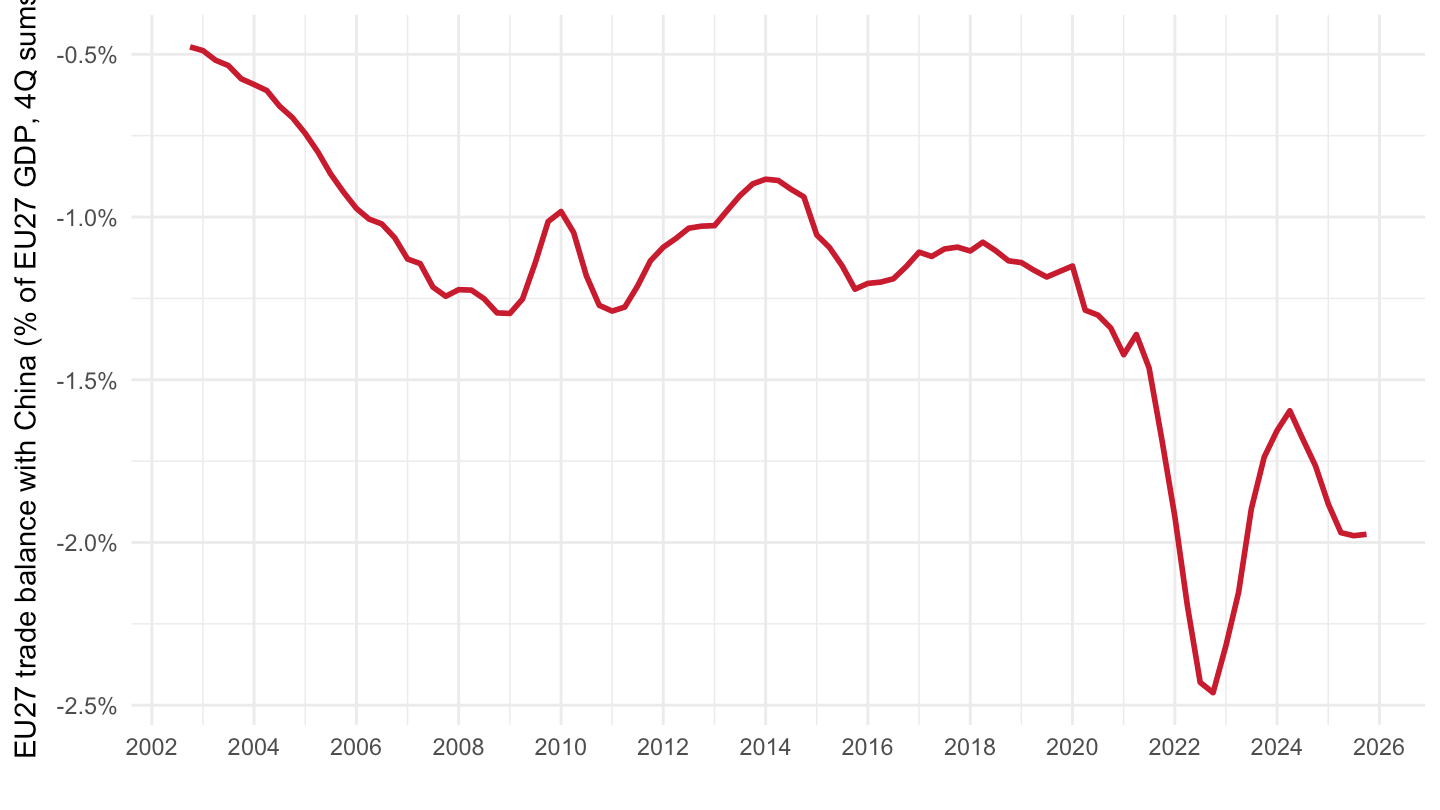
q_first <- as.Date("2002-10-01")  # first quarter with a full 4-quarter window
q_last  <- max(cn_q$date)

cn_q |>
  filter(date %in% c(q_first, q_last)) |>
  mutate(flow = recode(stk_flow, EXP = "Exports", IMP = "Imports"),
         period = factor(paste0(format(date, "%Y"), "Q", quarter(date)))) |>
  ggplot(aes(x = flow, y = pct_gdp, fill = period)) +
  geom_col(position = "dodge") +
  geom_text(aes(label = sprintf("%.1f%%", pct_gdp)),
            position = position_dodge(width = 0.9), vjust = -0.4) +
  theme_minimal() +
  scale_fill_manual(values = c("#7A7A7A", "#C8102E")) +
  scale_y_continuous(labels = scales::percent_format(scale = 1, accuracy = 0.1),
                     expand = expansion(mult = c(0, 0.1))) +
  theme(legend.position = c(0.15, 0.85), legend.title = element_blank()) +
  xlab("") + ylab("EU27 trade with China (% of EU27 GDP, 4Q sums)")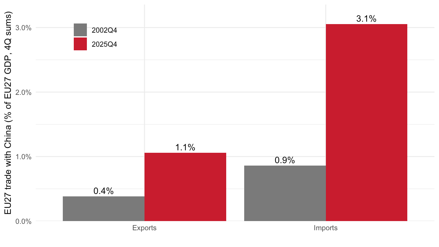
quarterly_trade("CN_X_HK", c("SITC5", "SITC6", "SITC7", "SITC8")) |>
  filter(stk_flow == "IMP") |>
  mutate(Sitc06 = paste0(sitc06, " - ", str_trunc(Sitc06, 30))) |>
  ggplot() + geom_area(aes(x = date, y = pct_gdp, fill = Sitc06)) +
  theme_minimal() +
  scale_x_date(breaks = as.Date(paste0(seq(2002, 2100, 2), "-01-01")),
               labels = date_format("%Y")) +
  scale_y_continuous(labels = scales::percent_format(scale = 1, accuracy = 0.1)) +
  theme(legend.position = "bottom", legend.title = element_blank()) +
  guides(fill = guide_legend(nrow = 2)) +
  xlab("") + ylab("EU27 imports from China (% of EU27 GDP, 4Q sums)")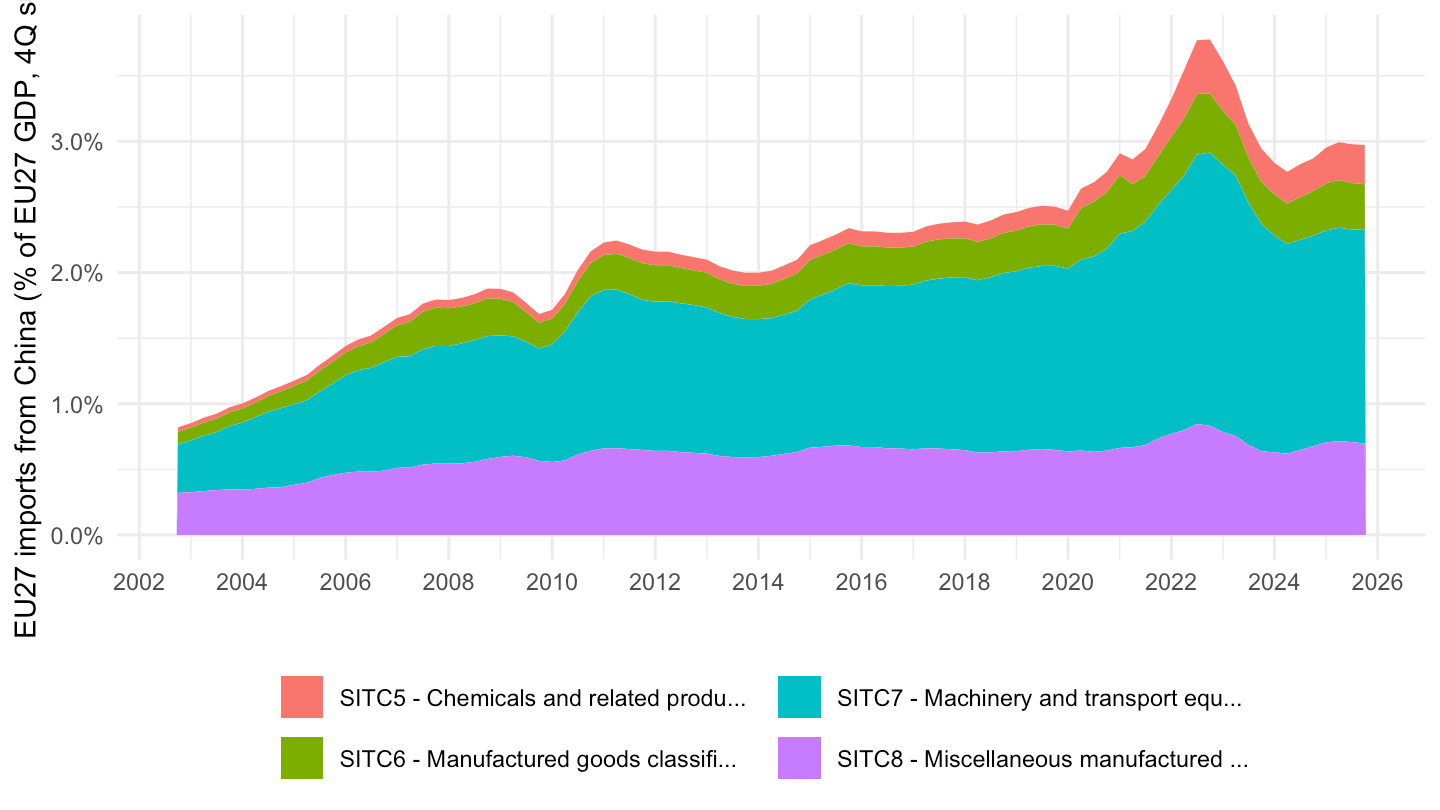
quarterly_trade(c("CN_X_HK", "US", "UK", "JP"), "SITC5-8") |>
  filter(stk_flow == "IMP") |>
  ggplot() + geom_line(aes(x = date, y = pct_gdp, color = Partner), linewidth = 1) +
  theme_minimal() +
  scale_x_date(breaks = as.Date(paste0(seq(2002, 2100, 2), "-01-01")),
               labels = date_format("%Y")) +
  scale_y_continuous(labels = scales::percent_format(scale = 1, accuracy = 0.1)) +
  theme(legend.position = c(0.2, 0.8), legend.title = element_blank()) +
  xlab("") + ylab("EU27 manufactured imports (% of EU27 GDP, 4Q sums)")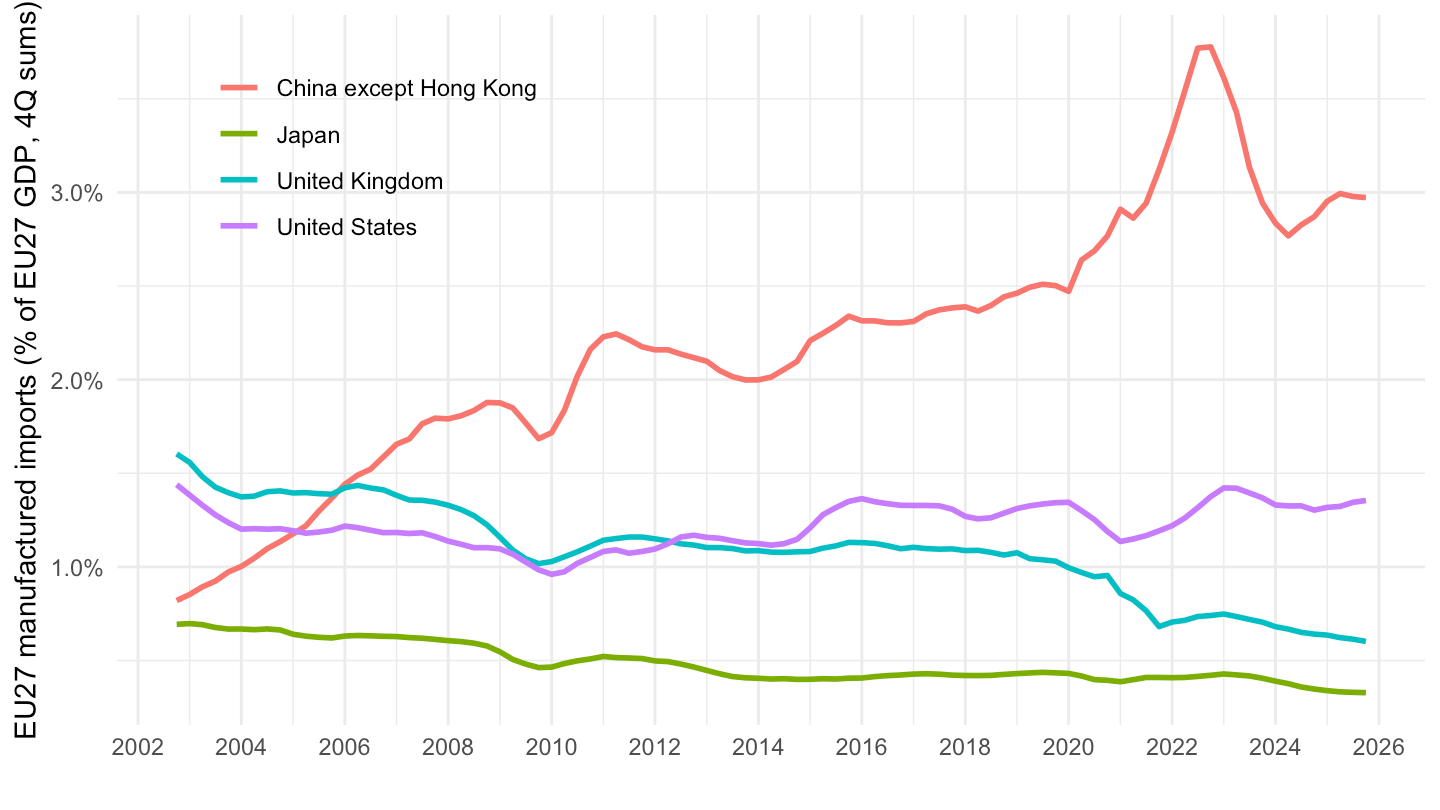
The “first” China shock (2001-2010 in the US literature) was followed by a second wave from the late 2010s: China moved up the value chain towards machinery, vehicles and electrical equipment (SITC 7), and since 2025 goods diverted from the US market are partly re-routed towards Europe.
share_partner <- annual_trade(c("CN_X_HK", "EXT_EU27_2020")) |>
  select(partner, stk_flow, year, values) |>
  pivot_wider(names_from = partner, values_from = values) |>
  mutate(share = 100 * CN_X_HK / EXT_EU27_2020,
         flow = recode(stk_flow, EXP = "Share in extra-EU27 exports",
                       IMP = "Share in extra-EU27 imports"))

share_partner |>
  ggplot() + geom_line(aes(x = year, y = share, color = flow), linewidth = 1) +
  geom_point(aes(x = year, y = share, color = flow)) +
  theme_minimal() +
  scale_x_continuous(breaks = seq(2002, 2100, 2)) +
  scale_y_continuous(labels = scales::percent_format(scale = 1, accuracy = 1)) +
  theme(legend.position = c(0.3, 0.85), legend.title = element_blank()) +
  xlab("") + ylab("China (excl. Hong Kong), % of extra-EU27 trade")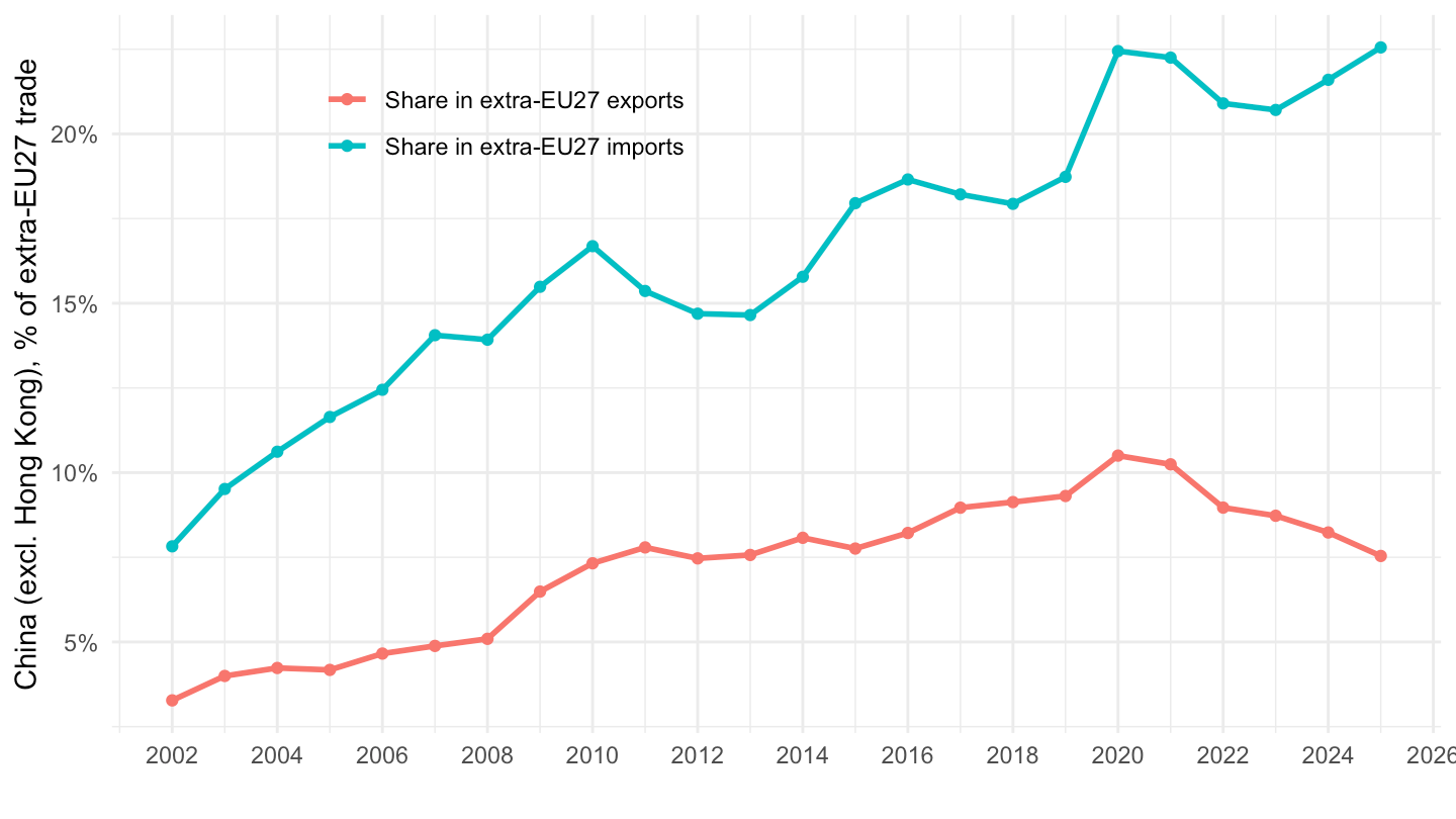
sh_sitc <- annual_trade(c("CN_X_HK", "EXT_EU27_2020"), sitc_main) |>
  filter(stk_flow == "IMP") |>
  select(partner, sitc06, Sitc06, year, values) |>
  pivot_wider(names_from = partner, values_from = values) |>
  mutate(share = 100 * CN_X_HK / EXT_EU27_2020,
         Sitc06 = paste0(sitc06, " - ", str_trunc(Sitc06, 30)))

sh_sitc |>
  filter(sitc06 %in% c("SITC5", "SITC6", "SITC7", "SITC8")) |>
  ggplot() + geom_line(aes(x = year, y = share, color = Sitc06), linewidth = 1) +
  theme_minimal() +
  scale_x_continuous(breaks = seq(2002, 2100, 2)) +
  scale_y_continuous(labels = scales::percent_format(scale = 1, accuracy = 1)) +
  theme(legend.position = "right", legend.title = element_blank()) +
  xlab("") + ylab("China (excl. HK), % of extra-EU27 imports")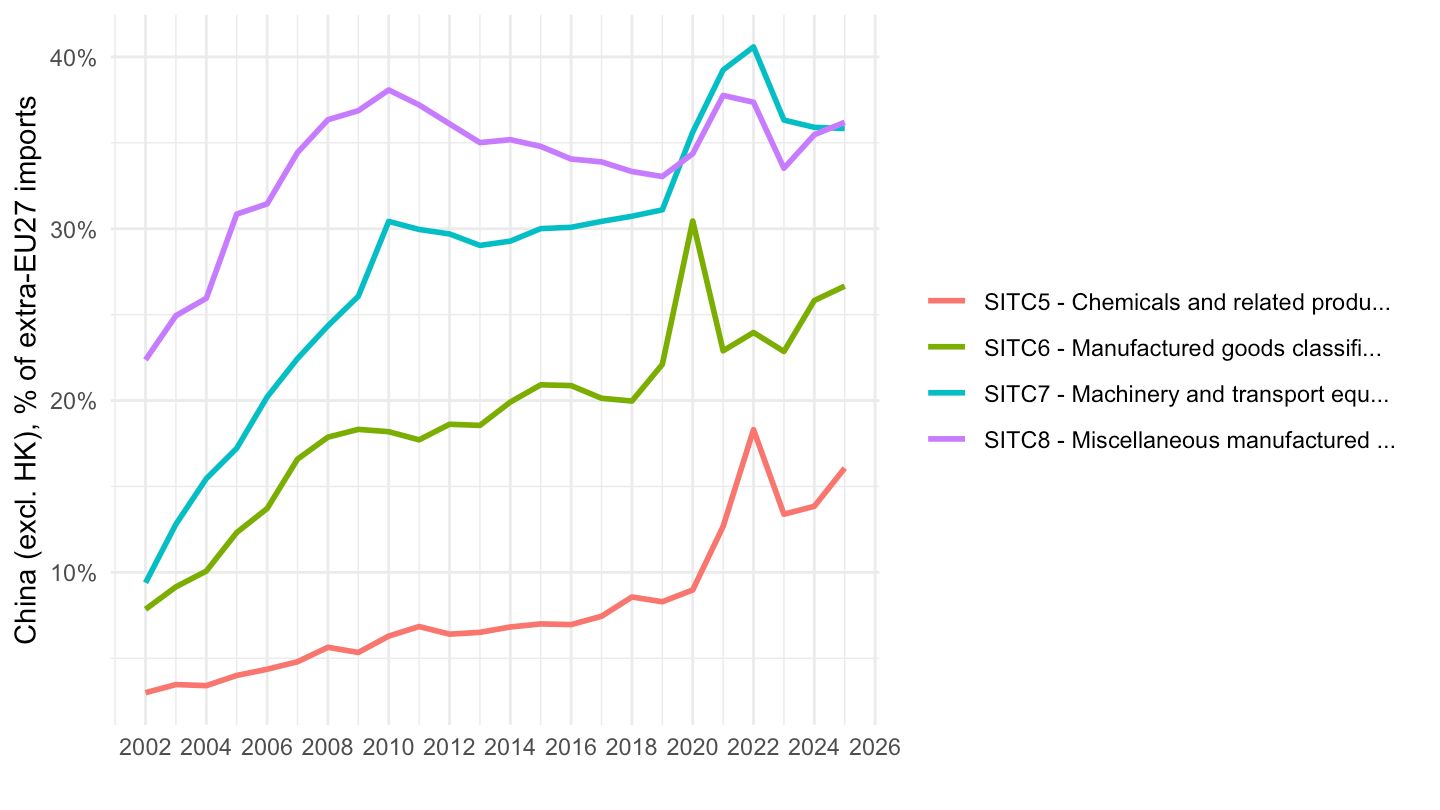
annual_trade(c("CN_X_HK", "US", "UK", "JP"), "SITC5-8") |>
  filter(stk_flow == "IMP") |>
  ggplot() + geom_line(aes(x = year, y = pct_gdp, color = Partner), linewidth = 1) +
  theme_minimal() +
  scale_x_continuous(breaks = seq(2002, 2100, 2)) +
  scale_y_continuous(labels = scales::percent_format(scale = 1, accuracy = 0.1)) +
  theme(legend.position = c(0.2, 0.8), legend.title = element_blank()) +
  xlab("") + ylab("EU27 imports of manufactured goods (% of EU27 GDP)")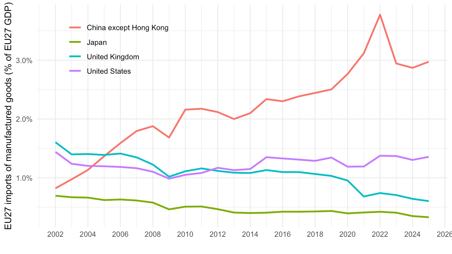
annual_trade("CN_X_HK", "SITC7") |>
  mutate(flow = recode(stk_flow, EXP = "Exports to China", IMP = "Imports from China")) |>
  ggplot() + geom_line(aes(x = year, y = pct_gdp, color = flow), linewidth = 1) +
  theme_minimal() +
  scale_x_continuous(breaks = seq(2002, 2100, 2)) +
  scale_y_continuous(labels = scales::percent_format(scale = 1, accuracy = 0.1)) +
  theme(legend.position = c(0.2, 0.8), legend.title = element_blank()) +
  xlab("") + ylab("EU27 trade in machinery & transport eq. (% of EU27 GDP)")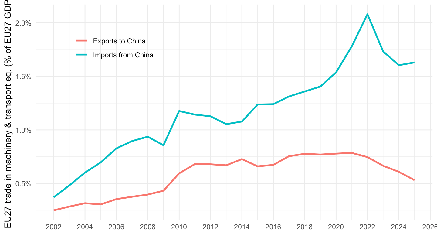
ext_st_eu27_2020sitc |>
  filter(stk_flow %in% c("EXP", "IMP"),
         indic_et == "TRD_VAL",
         sitc06 == "TOTAL",
         partner == "CN_X_HK") |>
  month_to_date() |>
  arrange(stk_flow, date) |>
  group_by(stk_flow) |>
  mutate(roll12 = zoo::rollsum(values, 12, fill = NA, align = "right") / 1000,
         flow = recode(stk_flow, EXP = "Exports to China", IMP = "Imports from China")) |>
  ungroup() |>
  filter(!is.na(roll12)) |>
  ggplot() + geom_line(aes(x = date, y = roll12, color = flow), linewidth = 1) +
  theme_minimal() +
  scale_x_date(breaks = as.Date(paste0(seq(2002, 2100, 2), "-01-01")),
               labels = date_format("%Y")) +
  theme(legend.position = c(0.2, 0.8), legend.title = element_blank()) +
  xlab("") + ylab("EU27 trade with China, 12-month sum (Bn€)")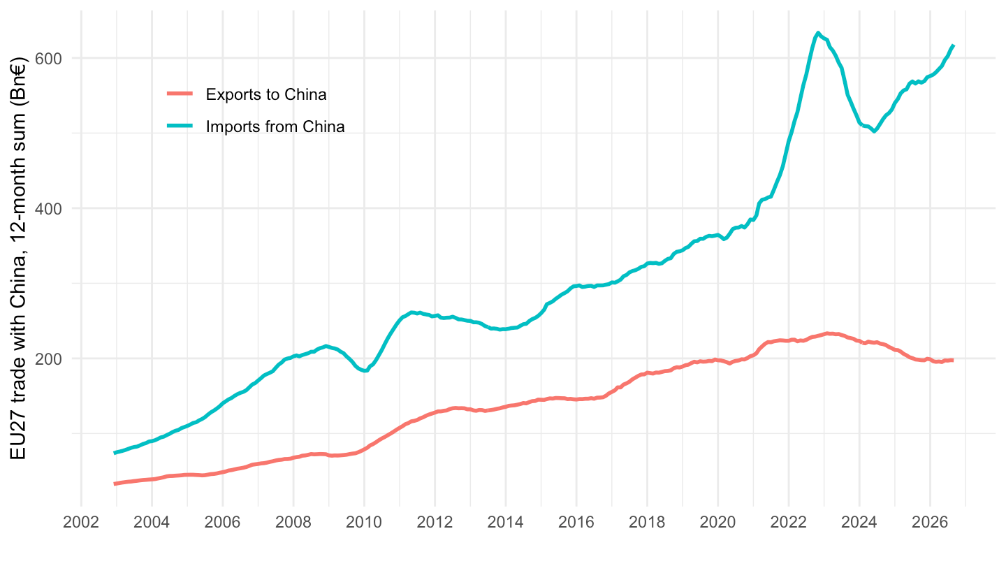
ext_st_eu27_2020sitc |>
  filter(stk_flow == "IMP",
         indic_et == "TRD_VAL",
         sitc06 == "TOTAL",
         partner %in% c("CN_X_HK", "US")) |>
  month_to_date() |>
  arrange(partner, date) |>
  group_by(Partner) |>
  mutate(yoy = 100 * (values / lag(values, 12) - 1)) |>
  ungroup() |>
  filter(date >= as.Date("2023-01-01")) |>
  ggplot() + geom_line(aes(x = date, y = yoy, color = Partner), linewidth = 1) +
  geom_hline(yintercept = 0, linetype = "dashed") +
  theme_minimal() +
  scale_x_date(breaks = "6 months", labels = date_format("%b %Y")) +
  scale_y_continuous(labels = scales::percent_format(scale = 1)) +
  theme(legend.position = c(0.2, 0.2), legend.title = element_blank()) +
  xlab("") + ylab("EU27 imports, year-on-year change")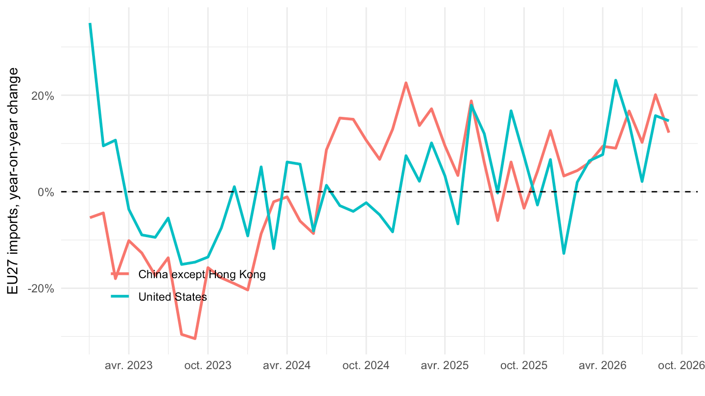
ext_st_eu27_2020sitc |>
  filter(stk_flow == "IMP",
         indic_et == "TRD_VAL",
         sitc06 %in% c("SITC7", "SITC8", "SITC6", "SITC5"),
         partner == "CN_X_HK") |>
  month_to_date() |>
  arrange(sitc06, date) |>
  group_by(sitc06, Sitc06) |>
  mutate(roll12 = zoo::rollsum(values, 12, fill = NA, align = "right"),
         base = mean(roll12[format(date, "%Y-%m") == "2019-12"]),
         index = 100 * roll12 / base) |>
  ungroup() |>
  filter(date >= as.Date("2019-12-01")) |>
  ggplot() + geom_line(aes(x = date, y = index, color = Sitc06), linewidth = 1) +
  geom_hline(yintercept = 100, linetype = "dashed") +
  theme_minimal() +
  scale_x_date(breaks = as.Date(paste0(2019:2100, "-12-01")), labels = date_format("%Y")) +
  theme(legend.position = "bottom", legend.title = element_blank()) +
  guides(color = guide_legend(nrow = 2)) +
  xlab("") + ylab("Imports from China, 12m sum (Dec 2019 = 100)")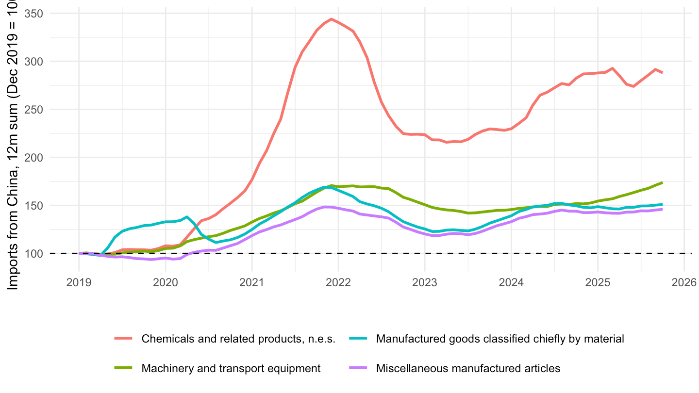
ext_st_eu27_2020sitc |>
  filter(stk_flow == "EXP",
         indic_et == "TRD_VAL",
         partner == "EXT_EU27_2020",
         sitc06 %in% c("SITC7", "SITC6", "SITC5", "SITC3")) |>
  month_to_date() |>
  mutate(values = values/1000) |>
  ggplot() + geom_line(aes(x = date, y = values, color = Sitc06)) +
  theme_minimal() +
  scale_x_date(breaks = as.Date(paste0(seq(2002, 2100, 2), "-01-01")),
               labels = date_format("%Y")) +
  theme(legend.position = "right") +
  xlab("") + ylab("EU27 exports to Extra-EU27 (Bn€)")
latest_m <- ext_st_eu27_2020sitc |>
  filter(stk_flow == "BAL_RT",
         indic_et == "TRD_VAL",
         sitc06 == "TOTAL",
         partner == "EXT_EU27_2020",
         !is.na(values)) |>
  summarise(m = max(time)) |>
  pull(m)

ext_st_eu27_2020sitc |>
  filter(stk_flow == "BAL_RT",
         indic_et == "TRD_VAL",
         sitc06 == "TOTAL",
         partner %in% c("EXT_EU27_2020", "US", "CN_X_HK", "UK", "JP"),
         time == latest_m) |>
  mutate(values = values/1000) |>
  select(partner, Partner, values) |>
  arrange(values) |>
print_table_conditional()| partner | Partner | values |
|---|---|---|
| CN_X_HK | China except Hong Kong | -41.7362 |
| EXT_EU27_2020 | Extra-EU27 (from 2020) | -16.7858 |
| JP | Japan | 0.0446 |
| US | United States | 10.9050 |
| UK | United Kingdom | 18.7111 |