Code
tibble(LAST_DOWNLOAD = as.Date(file.info("~/iCloud/website/data/eurostat/edat_lfs_9903.RData")$mtime)) %>%
print_table_conditional()| LAST_DOWNLOAD |
|---|
| 2026-02-03 |
Data - Eurostat
tibble(LAST_DOWNLOAD = as.Date(file.info("~/iCloud/website/data/eurostat/edat_lfs_9903.RData")$mtime)) %>%
print_table_conditional()| LAST_DOWNLOAD |
|---|
| 2026-02-03 |
| LAST_COMPILE |
|---|
| 2026-07-24 |
edat_lfs_9903 %>%
  group_by(time) %>%
  summarise(Nobs = n()) %>%
  arrange(desc(time)) %>%
  head(1) %>%
print_table_conditional()| time | Nobs |
|---|---|
| 2024 | 17496 |
edat_lfs_9903 %>%
  left_join(unit, by = "unit") %>%
  group_by(unit, Unit) %>%
  summarise(Nobs = n()) %>%
  arrange(-Nobs) %>%
print_table_conditional()| unit | Unit | Nobs |
|---|---|---|
| PC | Percentage | 273408 |
edat_lfs_9903 %>%
  left_join(sex, by = "sex") %>%
  group_by(sex, Sex) %>%
  summarise(Nobs = n()) %>%
  arrange(-Nobs) %>%
print_table_conditional()| sex | Sex | Nobs |
|---|---|---|
| F | Females | 91136 |
| M | Males | 91136 |
| T | Total | 91136 |
edat_lfs_9903 %>%
  left_join(age, by = "age") %>%
  group_by(age, Age) %>%
  summarise(Nobs = n()) %>%
  arrange(-Nobs) %>%
print_table_conditional()| age | Age | Nobs |
|---|---|---|
| Y15-19 | From 15 to 19 years | 11472 |
| Y15-24 | From 15 to 24 years | 11472 |
| Y15-29 | From 15 to 29 years | 11472 |
| Y18-24 | From 18 to 24 years | 11472 |
| Y20-24 | From 20 to 24 years | 11472 |
| Y20-29 | From 20 to 29 years | 11472 |
| Y25-29 | From 25 to 29 years | 11472 |
| Y25-34 | From 25 to 34 years | 11472 |
| Y15-64 | From 15 to 64 years | 9924 |
| Y15-69 | From 15 to 69 years | 9924 |
| Y15-74 | From 15 to 74 years | 9924 |
| Y18-64 | From 18 to 64 years | 9924 |
| Y18-69 | From 18 to 69 years | 9924 |
| Y18-74 | From 18 to 74 years | 9924 |
| Y25-54 | From 25 to 54 years | 9924 |
| Y25-64 | From 25 to 64 years | 9924 |
| Y25-69 | From 25 to 69 years | 9924 |
| Y25-74 | From 25 to 74 years | 9924 |
| Y30-54 | From 30 to 54 years | 9924 |
| Y35-44 | From 35 to 44 years | 9924 |
| Y35-54 | From 35 to 54 years | 9924 |
| Y45-54 | From 45 to 54 years | 9924 |
| Y55-64 | From 55 to 64 years | 9924 |
| Y55-69 | From 55 to 69 years | 9924 |
| Y55-74 | From 55 to 74 years | 9924 |
| Y30-34 | From 30 to 34 years | 7236 |
| Y45-64 | From 45 to 64 years | 5688 |
load_data("eurostat/isced11_fr.RData")
edat_lfs_9903 %>%
  left_join(isced11, by = "isced11") %>%
  group_by(isced11, Isced11) %>%
  summarise(Nobs = n()) %>%
  arrange(-Nobs) %>%
print_table_conditional()| isced11 | Isced11 | Nobs |
|---|---|---|
| ED0-2 | Inférieur à l'enseignement primaire, enseignement primaire et premier cycle de l'enseignement secondaire (niveaux 0-2) | 59037 |
| ED3-8 | Deuxième cycle de l'enseignement secondaire, enseignement post-secondaire non-supérieur et enseignement supérieur (niveaux 3-8) | 59037 |
| ED3_4 | Deuxième cycle de l'enseignement secondaire et enseignement post-secondaire non-supérieur (niveaux 3 et 4) | 59037 |
| ED5-8 | Enseignement supérieur (niveaux 5-8) | 59037 |
| ED34_44 | Deuxième cycle du secondaire et post-secondaire non-supérieur - général (niveaux 34 et 44) | 18630 |
| ED35_45 | Deuxième cycle du secondaire et post-secondaire non-supérieur - professionnel (niveaux 35 et 45) | 18630 |
edat_lfs_9903 %>%
  left_join(geo, by = "geo") %>%
  group_by(geo, Geo) %>%
  summarise(Nobs = n()) %>%
  arrange(-Nobs) %>%
  mutate(Geo = ifelse(geo == "DE", "Germany", Geo)) %>%
  mutate(Flag = gsub(" ", "-", str_to_lower(Geo)),
         Flag = paste0('<img src="../../icon/flag/vsmall/', Flag, '.png" alt="Flag">')) %>%
  select(Flag, everything()) %>%
{if (is_html_output()) datatable(., filter = 'top', rownames = F, escape = F) else .}edat_lfs_9903 %>%
group_by(time) %>%
summarise(Nobs = n()) %>%
arrange(desc(time)) %>%
print_table_conditional()| time | Nobs |
|---|---|
| 2024 | 17496 |
| 2023 | 17496 |
| 2022 | 17496 |
| 2021 | 17496 |
| 2020 | 13608 |
| 2019 | 13986 |
| 2018 | 13986 |
| 2017 | 13986 |
| 2016 | 13986 |
| 2015 | 13986 |
| 2014 | 13986 |
| 2013 | 11100 |
| 2012 | 11100 |
| 2011 | 11100 |
| 2010 | 10800 |
| 2009 | 10500 |
| 2008 | 10500 |
| 2007 | 10500 |
| 2006 | 10500 |
| 2005 | 9900 |
| 2004 | 9900 |
edat_lfs_9903 %>%
  filter(isced11 == "ED0-2",
         age == "Y15-74",
         geo %in% c("EA19", "DE", "ES", "FR", "IT"),
         sex == "T") %>%
  select_if(~ n_distinct(.) > 1) %>%
  year_to_date() %>%
  filter(date >= as.Date("1995-01-01")) %>%
  left_join(geo, by = "geo") %>%
  mutate(Geo = ifelse(geo == "DE", "Germany", Geo)) %>%
  mutate(Geo = ifelse(geo == "EA19", "Europe", Geo)) %>%
  left_join(colors, by = c("Geo" = "country")) %>%
  mutate(color = ifelse(geo == "EA19", color2, color)) %>%
  mutate(color = ifelse(geo == "ES", color2, color)) %>%
  mutate(values = values / 100) %>%
  ggplot(.) + geom_line(aes(x = date, y = values, color = color)) +
  theme_minimal() + xlab("") + ylab("% Population du 1er cycle de l'enseignement secondaire") +
  scale_color_identity() + add_5flags +
  scale_x_date(breaks = seq(1960, 2100, 5) %>% paste0("-01-01") %>% as.Date,
               labels = date_format("%Y")) +
  scale_y_continuous(breaks = 0.01*seq(-500, 200, 2),
                     labels = percent_format(accuracy = 1))
edat_lfs_9903 %>%
  filter(isced11 == "ED3_4",
         age == "Y15-74",
         geo %in% c("EA19", "DE", "ES", "FR", "IT"),
         sex == "T") %>%
  year_to_date() %>%
  filter(date >= as.Date("1995-01-01")) %>%
  left_join(geo, by = "geo") %>%
  mutate(Geo = ifelse(geo == "DE", "Germany", Geo)) %>%
  mutate(Geo = ifelse(geo == "EA19", "Europe", Geo)) %>%
  left_join(colors, by = c("Geo" = "country")) %>%
  mutate(color = ifelse(geo == "EA19", color2, color)) %>%
  mutate(color = ifelse(geo == "ES", color2, color)) %>%
  mutate(values = values / 100) %>%
  ggplot(.) + geom_line(aes(x = date, y = values, color = color)) +
  theme_minimal() + xlab("") + ylab("% Population des niveaux 3 et 4") +
  scale_color_identity() + add_5flags +
  scale_x_date(breaks = seq(1960, 2100, 5) %>% paste0("-01-01") %>% as.Date,
               labels = date_format("%Y")) +
  scale_y_continuous(breaks = 0.01*seq(-500, 200, 2),
                     labels = percent_format(accuracy = 1))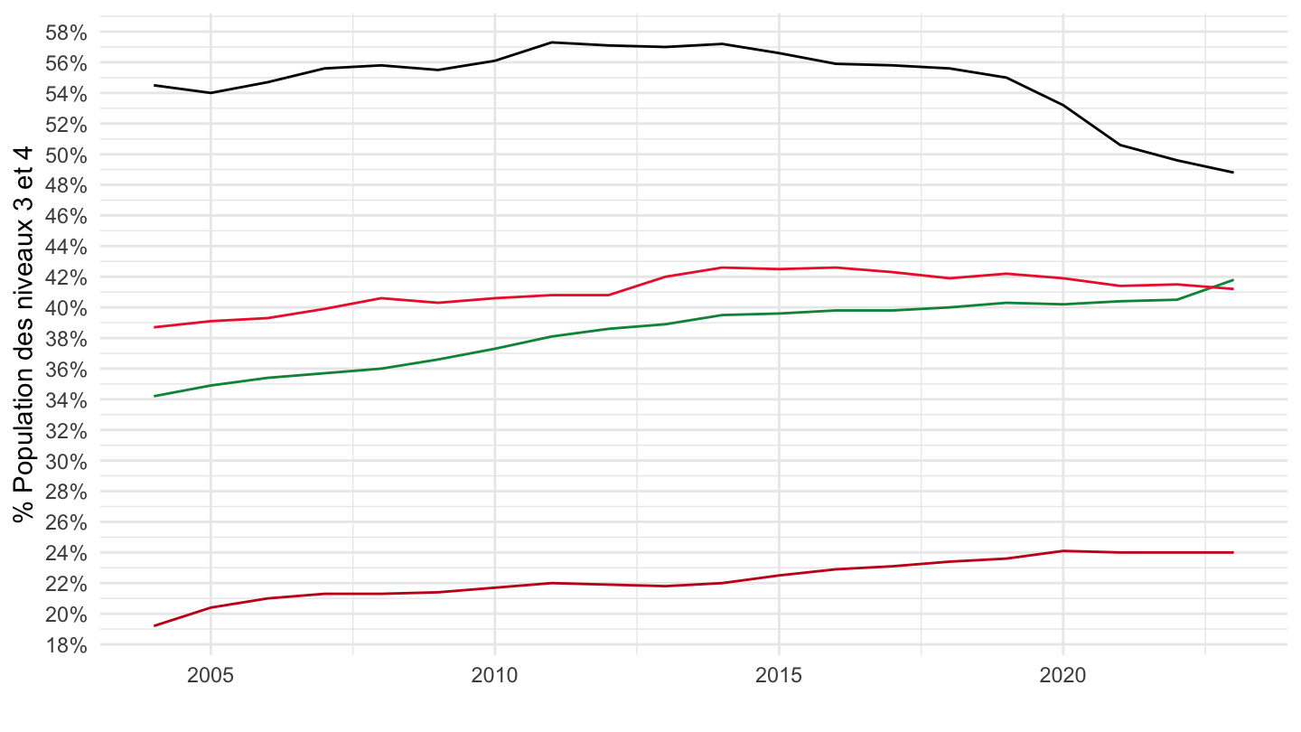
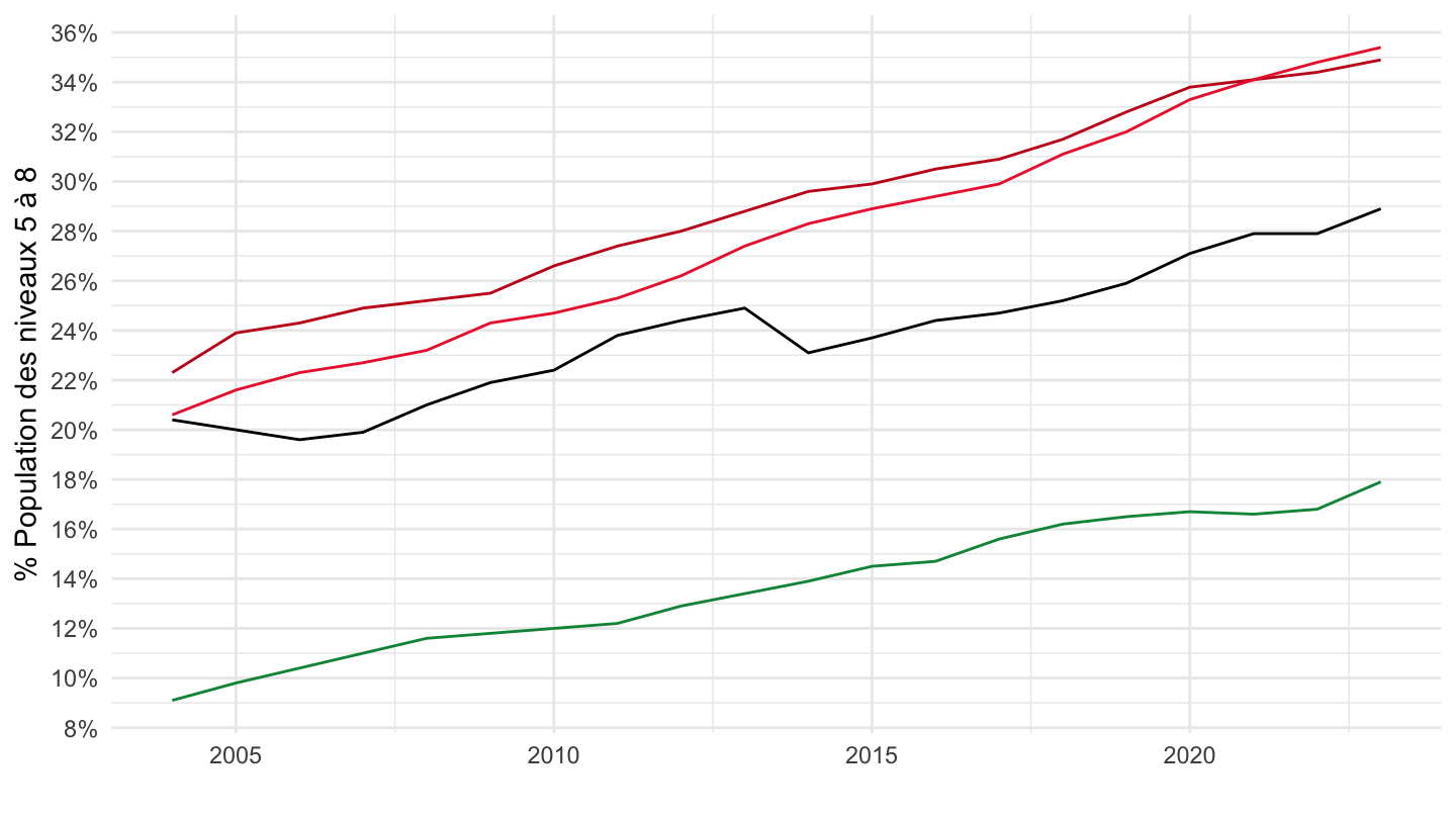
edat_lfs_9903 %>%
  filter(isced11 == "ED5-8",
         age == "Y15-74",
         geo %in% c("EA19", "DE", "ES", "FR", "IT"),
         sex == "T") %>%
  year_to_date() %>%
  filter(date >= as.Date("1995-01-01")) %>%
  left_join(geo, by = "geo") %>%
  mutate(Geo = ifelse(geo == "DE", "Germany", Geo)) %>%
  mutate(Geo = ifelse(geo == "EA19", "Europe", Geo)) %>%
  left_join(colors, by = c("Geo" = "country")) %>%
  mutate(color = ifelse(geo == "EA19", color2, color)) %>%
  mutate(color = ifelse(geo == "ES", color2, color)) %>%
  mutate(values = values / 100) %>%
  ggplot(.) + geom_line(aes(x = date, y = values, color = color)) +
  theme_minimal() + xlab("") + ylab("% Population des niveaux 5 à 8") +
  scale_color_identity() + add_5flags +
  scale_x_date(breaks = seq(1960, 2100, 5) %>% paste0("-01-01") %>% as.Date,
               labels = date_format("%Y")) +
  scale_y_continuous(breaks = 0.01*seq(-500, 200, 2),
                     labels = percent_format(accuracy = 1))