Structure of earnings survey - hourly earnings - earn_ses_hourly

Data - Eurostat

Info

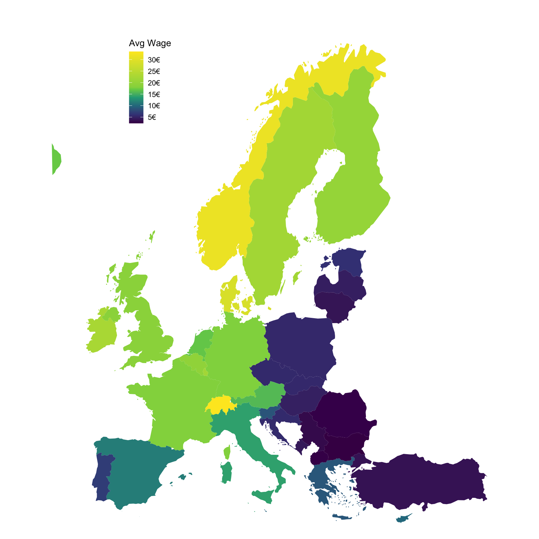
Last observation: Annual: 2022 (N = 200,970)

First observation: Annual: 2002 (N = 720,588)

Last data update: 11 aoû 2026, 21:05. Last compile: 11 aoû 2026, 23:29

Structure

freq

nace_r2

isco08

worktime

age

sex

indic_se

geo

Mean Hourly Earnings

France, Germany, Italy, Spain

earn_ses_hourly |>
  filter(geo %in% c("FR", "DE", "IT", "ES"),
         nace_r2 == "B-N",
         isco08 == "TOTAL",
         worktime == "TOTAL",
         age == "TOTAL",
         sex == "T",
         indic_se == "MEAN_E_EUR") |>
  year_to_date() |>
  left_join(colors, by = c("Geo" = "country")) |>
  ggplot() + geom_line(aes(x = date, y = values, color = color)) +
  theme_minimal() + scale_color_identity() + add_flags +
  scale_x_date(breaks = as.Date(paste0(seq(2000, 2100, 4), "-01-01")),
               labels = date_format("%Y")) +
  xlab("") + ylab("Mean hourly earnings (€)")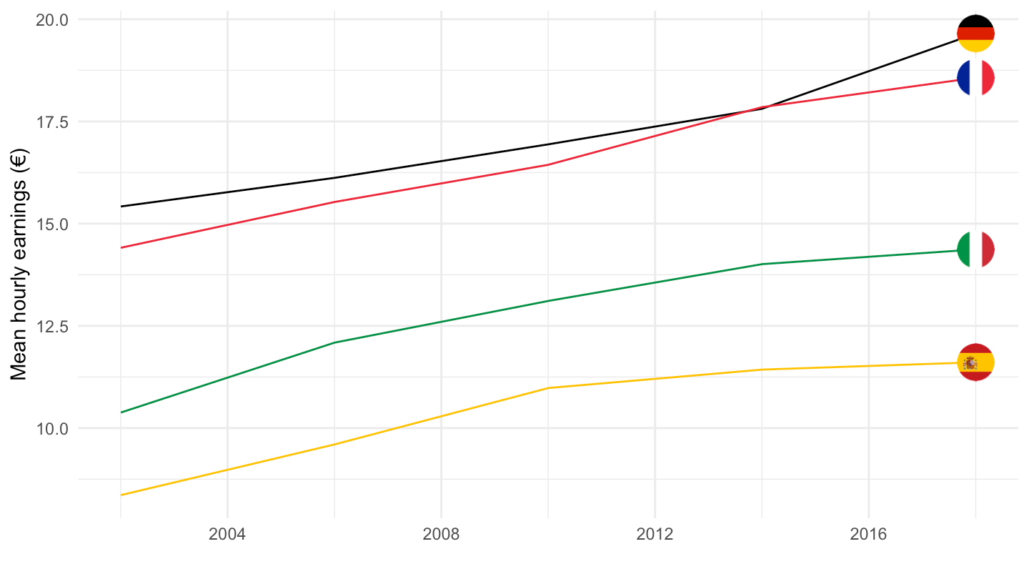

Gender Pay Gap

Unadjusted, France, Germany, Italy, Spain

earn_ses_hourly |>
  filter(geo %in% c("FR", "DE", "IT", "ES"),
         nace_r2 == "B-N",
         isco08 == "TOTAL",
         worktime == "TOTAL",
         age == "TOTAL",
         sex %in% c("M", "F"),
         indic_se == "MEAN_E_EUR") |>
  select(geo, Geo, time, sex, values) |>
  spread(sex, values) |>
  mutate(values = (M - F)/M) |>
  year_to_date() |>
  left_join(colors, by = c("Geo" = "country")) |>
  ggplot() + geom_line(aes(x = date, y = values, color = color)) +
  theme_minimal() + scale_color_identity() + add_flags +
  scale_x_date(breaks = as.Date(paste0(seq(2000, 2100, 4), "-01-01")),
               labels = date_format("%Y")) +
  xlab("") + ylab("Gender pay gap, unadjusted (mean, B-N)") +
  scale_y_continuous(labels = scales::percent_format(accuracy = 1)) +
  geom_hline(yintercept = 0, linetype = "dashed", color = "black")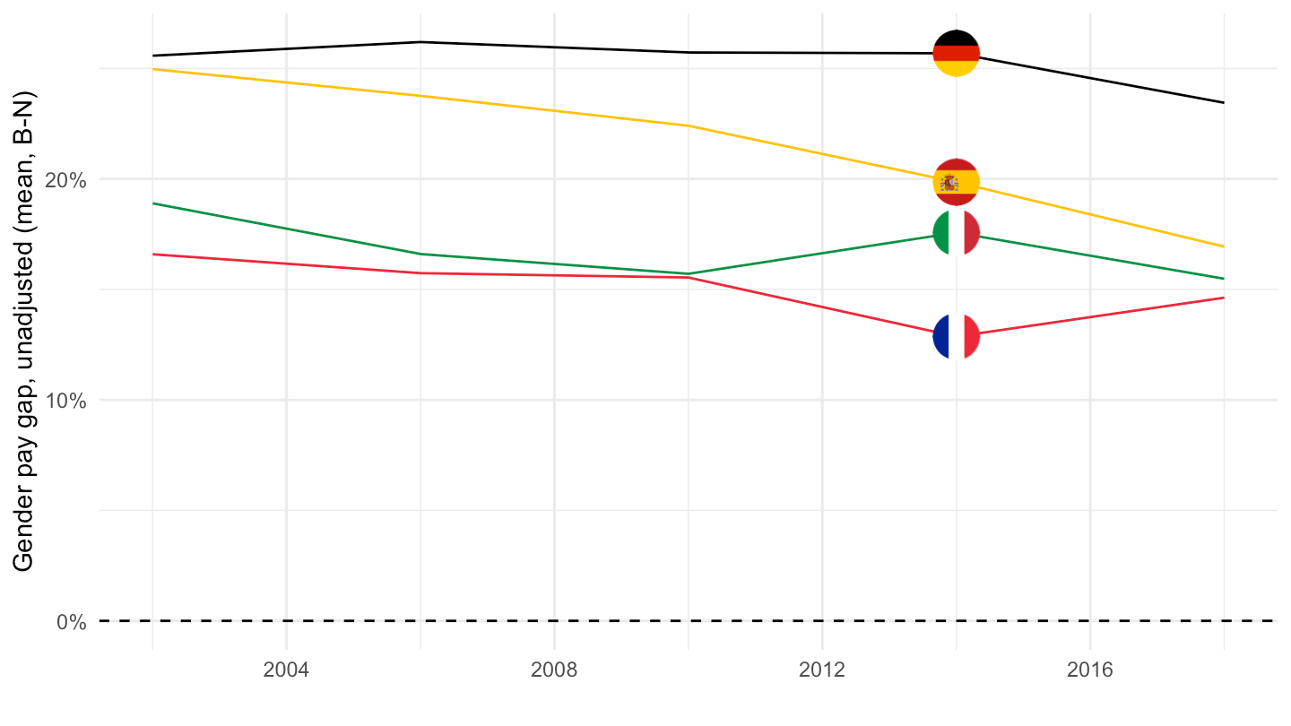

Table

png

include_graphics3b("bib/eurostat/earn_ses_hourly_ex1.png")

Javascript

earn_ses_hourly |>
  filter(nace_r2 == "B-N",
         isco08 == "TOTAL",
         worktime == "TOTAL", 
         age == "TOTAL",
         sex == "T",
         indic_se == "MEAN_E_EUR",
         time %in% c("2002", "2010", "2018")) |>
  
  select(geo, Geo, time, values) |>
  na.omit() |>
  mutate(Geo = ifelse(geo == "DE", "Germany", Geo),
         values = round(values)) |>
  spread(time, values) %>%
  mutate_at(vars(-1, -2), funs(ifelse(is.na(.), "", paste0(., " €")))) %>%
  {if (is_html_output()) datatable(., filter = 'top', rownames = F) else .}

Maps

2018

earn_ses_hourly |>
  filter(nace_r2 == "B-N",
         isco08 == "TOTAL",
         worktime == "TOTAL", 
         age == "TOTAL",
         sex == "T",
         indic_se == "MEAN_E_EUR",
         time %in% c("2018")) |>
  
  select(geo, Geo, values) |>
  right_join(europe_NUTS0, by = "geo") |>
  filter(long >= -15, lat >= 33) |>
  ggplot(aes(x = long, y = lat, group = group, fill = values)) +
  geom_polygon() + coord_map() +
  scale_fill_viridis_c(na.value = "white",
                       labels = scales::dollar_format(accuracy = 1, prefix = "", suffix = "€"),
                       breaks = seq(0, 100, 5),
                       values = c(0, 0.1, 0.2, 0.3, 0.4, 0.5, 1)) +
  theme_void() + theme(legend.position = c(0.25, 0.85)) + 
  labs(fill = "Avg Wage")

2014

earn_ses_hourly |>
  filter(nace_r2 == "B-N",
         isco08 == "TOTAL",
         worktime == "TOTAL", 
         age == "TOTAL",
         sex == "T",
         indic_se == "MEAN_E_EUR",
         time %in% c("2014")) |>
  
  select(geo, Geo, values) |>
  right_join(europe_NUTS0, by = "geo") |>
  filter(long >= -15, lat >= 33) |>
  ggplot(aes(x = long, y = lat, group = group, fill = values)) +
  geom_polygon() + coord_map() +
  scale_fill_viridis_c(na.value = "white",
                       labels = scales::dollar_format(accuracy = 1, prefix = "", suffix = "€"),
                       breaks = seq(0, 100, 5),
                       values = c(0, 0.1, 0.2, 0.3, 0.4, 0.5, 1)) +
  theme_void() + theme(legend.position = c(0.25, 0.85)) + 
  labs(fill = "Avg Wage")