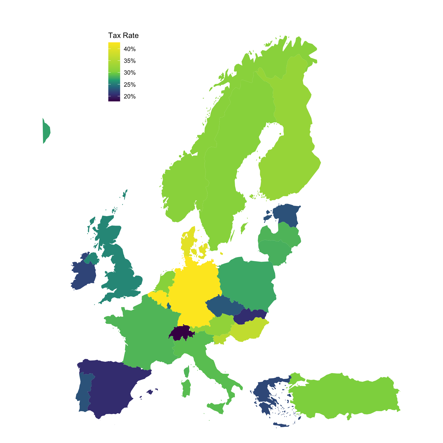
Last observation: 2025 (N = 390)
First observation: 2000 (N = 390)
Last data update: 04 oct. 2026, 22:52
Last compile: 09 oct. 2026, 22:13
earn_nt_taxrate |>
  filter(geo %in% c("FR", "DE", "IT", "ES", "PT"),
         ecase == "P1_NCH_AW100") |>
  year_to_date() |>

  add_flag_color("Geo") |>
  mutate(values = values/100) |>
  ggplot() + geom_line(aes(x = date, y = values, color = color)) +
  theme_minimal() + scale_color_identity() + add_flags +
  scale_x_date(breaks = as.Date(paste0(seq(2000, 2100, 2), "-01-01")),
               labels = date_format("%Y")) +
  xlab("") + ylab("Tax rate, single person, 100% of average earning") +
  scale_y_continuous(labels = scales::percent_format(accuracy = 1))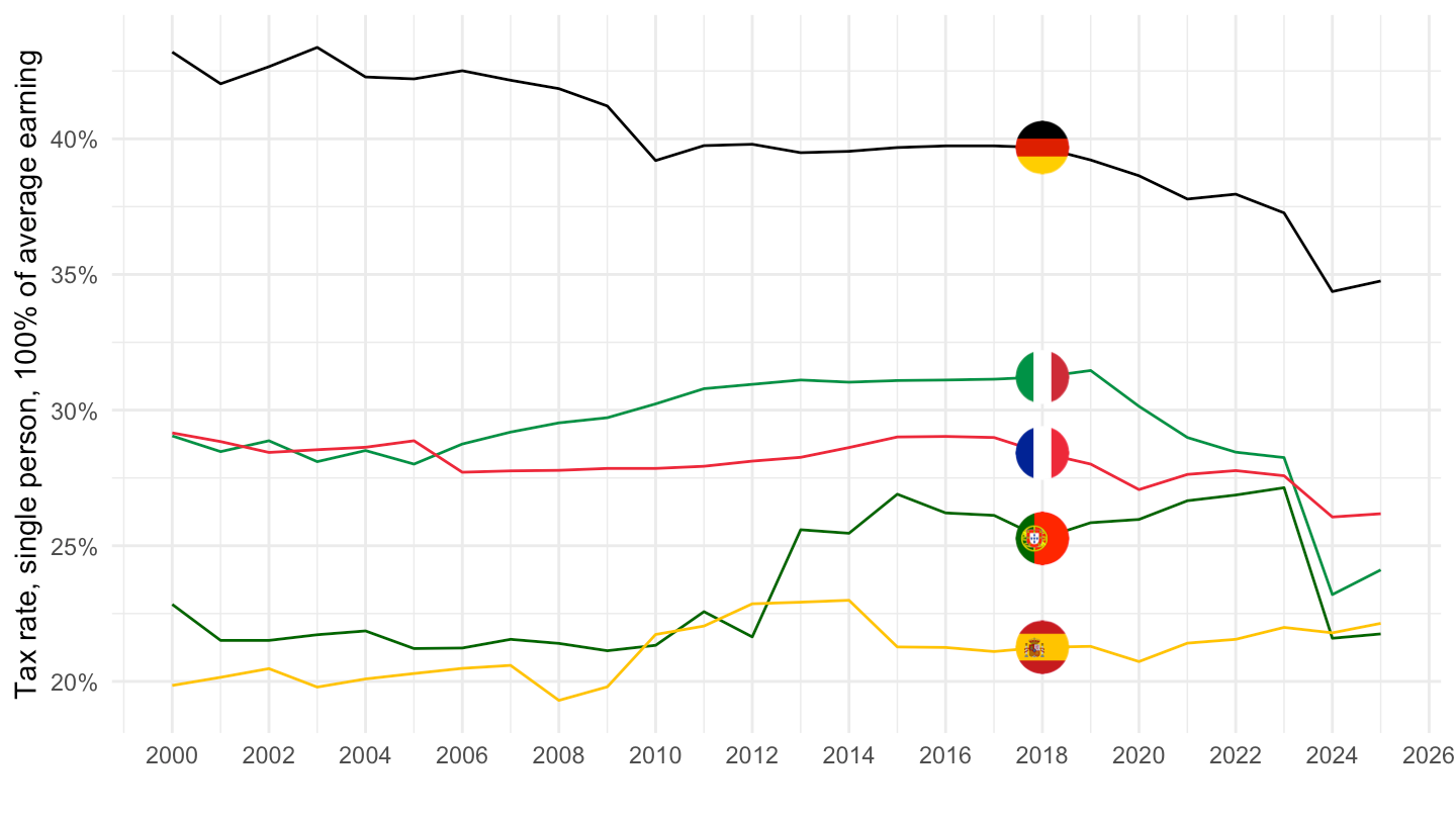
earn_nt_taxrate |>
  filter(geo == "FR",
         ecase %in% c("P1_NCH_AW67", "P1_NCH_AW100", "P1_NCH_AW167",
                       "CPL_NCH_AW100_33", "CPL_NCH_AW100_100")) |>
  year_to_date() |>
  mutate(values = values/100) |>
  ggplot() + geom_line(aes(x = date, y = values, color = Ecase)) +
  theme_minimal() +
  scale_x_date(breaks = as.Date(paste0(seq(2000, 2100, 2), "-01-01")),
               labels = date_format("%Y")) +
  xlab("") + ylab("Tax rate") +
  scale_y_continuous(labels = scales::percent_format(accuracy = 1)) +
  theme(legend.position = "right")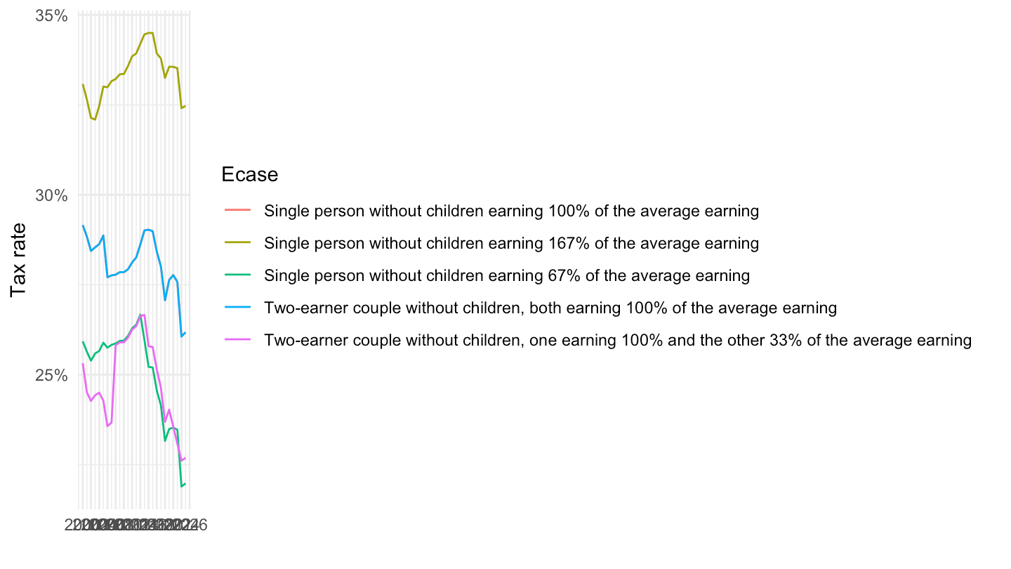
latest_y <- earn_nt_taxrate |>
  filter(ecase == "P1_NCH_AW100",
         geo == "FR",
         !is.na(values)) |>
  summarise(m = max(time)) |>
  pull(m)

earn_nt_taxrate |>
  filter(geo %in% c("FR", "DE", "IT", "ES", "PT", "EA20"),
         ecase %in% c("P1_NCH_AW67", "P1_NCH_AW100", "P1_NCH_AW167",
                       "CPL_NCH_AW100_33", "CPL_NCH_AW100_100"),
         time == latest_y) |>
  mutate(values = values/100) |>
  select(ecase, Ecase, Geo, values) |>
  spread(Geo, values) |>
print_table_conditional()| ecase | Ecase | Euro area – 20 countries (2023-2025) | France | Germany | Italy | Portugal | Spain |
|---|---|---|---|---|---|---|---|
| CPL_NCH_AW100_100 | Two-earner couple without children, both earning 100% of the average earning | 0.3083 | 0.2715 | 0.3702 | 0.3105 | 0.2435 | 0.2309 |
| CPL_NCH_AW100_33 | Two-earner couple without children, one earning 100% and the other 33% of the average earning | 0.2580 | 0.2337 | 0.3198 | 0.2401 | 0.1883 | 0.1948 |
| P1_NCH_AW100 | Single person without children earning 100% of the average earning | 0.3077 | 0.2715 | 0.3702 | 0.3105 | 0.2276 | 0.2291 |
| P1_NCH_AW167 | Single person without children earning 167% of the average earning | 0.3705 | 0.3302 | 0.4152 | 0.4015 | 0.3137 | 0.2913 |
| P1_NCH_AW67 | Single person without children earning 67% of the average earning | 0.2462 | 0.2270 | 0.3245 | 0.1976 | 0.1641 | 0.1827 |
earn_nt_taxrate |>
  filter(time == "2018",
         ecase == "P1_NCH_AW100") |>

  select(geo, Geo, values) |>
  right_join(europe_NUTS0, by = "geo") |>
  filter(long >= -15, lat >= 33) |>
  ggplot(aes(x = long, y = lat, group = group, fill = values/100)) +
  geom_polygon() + coord_map() +
  scale_fill_viridis_c(na.value = "white",
                       labels = scales::percent_format(a = 1),
                       breaks = 0.01*seq(0, 100, 5),
                       values = c(0, 0.1, 0.2, 0.3, 0.4, 0.5, 1)) +
  theme_void() + theme(legend.position = c(0.25, 0.85)) +
  labs(fill = "Tax Rate")
earn_nt_taxrate |>
  filter(time == "2002",
         ecase == "P1_NCH_AW100") |>

  select(geo, Geo, values) |>
  right_join(europe_NUTS0, by = "geo") |>
  filter(long >= -15, lat >= 33) |>
  ggplot(aes(x = long, y = lat, group = group, fill = values/100)) +
  geom_polygon() + coord_map() +
  scale_fill_viridis_c(na.value = "white",
                       labels = scales::percent_format(a = 1),
                       breaks = 0.01*seq(0, 100, 5),
                       values = c(0, 0.1, 0.2, 0.3, 0.4, 0.5, 1)) +
  theme_void() + theme(legend.position = c(0.25, 0.85)) +
  labs(fill = "Tax Rate")