Life expectancy by age, sex and NUTS 2 region - demo_r_mlifexp

Data - Eurostat

Author

unit

Code

demo_r_mlifexp %>%
  left_join(unit, by = "unit") %>%
  group_by(unit, Unit) %>%
  summarise(Nobs = n()) %>%
  arrange(-Nobs) %>%
  {if (is_html_output()) print_table(.) else .}

unit	Unit	Nobs
YR	Year	3330395

sex

Code

demo_r_mlifexp %>%
  left_join(sex, by = "sex") %>%
  group_by(sex, Sex) %>%
  summarise(Nobs = n()) %>%
  arrange(-Nobs) %>%
  {if (is_html_output()) print_table(.) else .}

sex	Sex	Nobs
T	Total	1110189
F	Females	1110103
M	Males	1110103

age

Code

demo_r_mlifexp %>%
  left_join(age, by = "age") %>%
  group_by(age, Age) %>%
  summarise(Nobs = n()) %>%
  arrange(-Nobs) %>%
  {if (is_html_output()) datatable(., filter = 'top', rownames = F) else .}

geo

Code

demo_r_mlifexp %>%
  left_join(geo, by = "geo") %>%
  group_by(geo, Geo) %>%
  summarise(Nobs = n()) %>%
  arrange(-Nobs) %>%
  {if (is_html_output()) datatable(., filter = 'top', rownames = F) else .}

NUTS 2 Life Expectancy

All

Code

demo_r_mlifexp %>%
  filter(time == "2018", 
         nchar(geo) == 4,
         sex == "T",
         age == "Y1") %>%
  left_join(geo, by = "geo") %>%
  select(geo, Geo, values) %>%
  right_join(europe_NUTS2, by = "geo") %>%
  filter(long >= -15, lat >= 33) %>%
  ggplot(., aes(x = long, y = lat, group = group, fill = values)) +
  geom_polygon() + coord_map() +
  scale_fill_viridis_c(na.value = "white",
                       direction = -1,
                       breaks = seq(70, 90, 2),
                       values = c(0, 0.1, 0.3, 0.5, 0.7, 0.9, 1)) +
  theme_void() + theme(legend.position = c(0.25, 0.85)) + 
  labs(fill = "Life Expectancy (Men and Women)")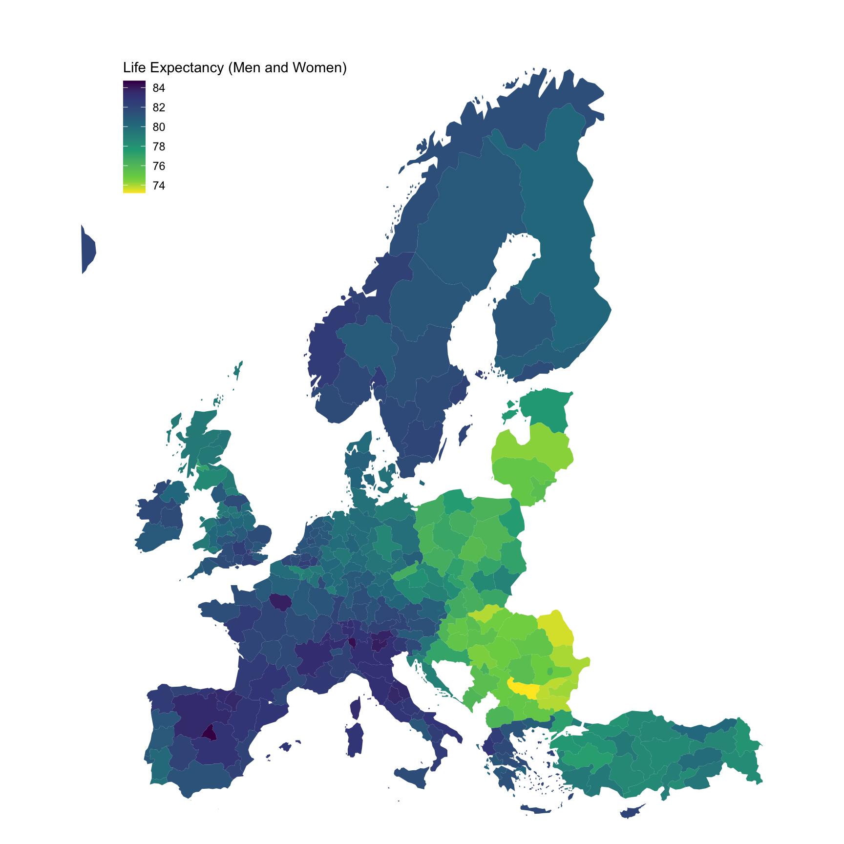

Men

Code

demo_r_mlifexp %>%
  filter(time == "2018", 
         nchar(geo) == 4,
         sex == "M",
         age == "Y1") %>%
  left_join(geo, by = "geo") %>%
  select(geo, Geo, values) %>%
  right_join(europe_NUTS2, by = "geo") %>%
  filter(long >= -15, lat >= 33) %>%
  ggplot(., aes(x = long, y = lat, group = group, fill = values)) +
  geom_polygon() + coord_map() +
  scale_fill_viridis_c(na.value = "white",
                       direction = -1,
                       breaks = seq(70, 90, 2),
                       values = c(0, 0.1, 0.3, 0.5, 0.7, 0.9, 1)) +
  theme_void() + theme(legend.position = c(0.25, 0.85)) + 
  labs(fill = "Life Expectancy (Men)")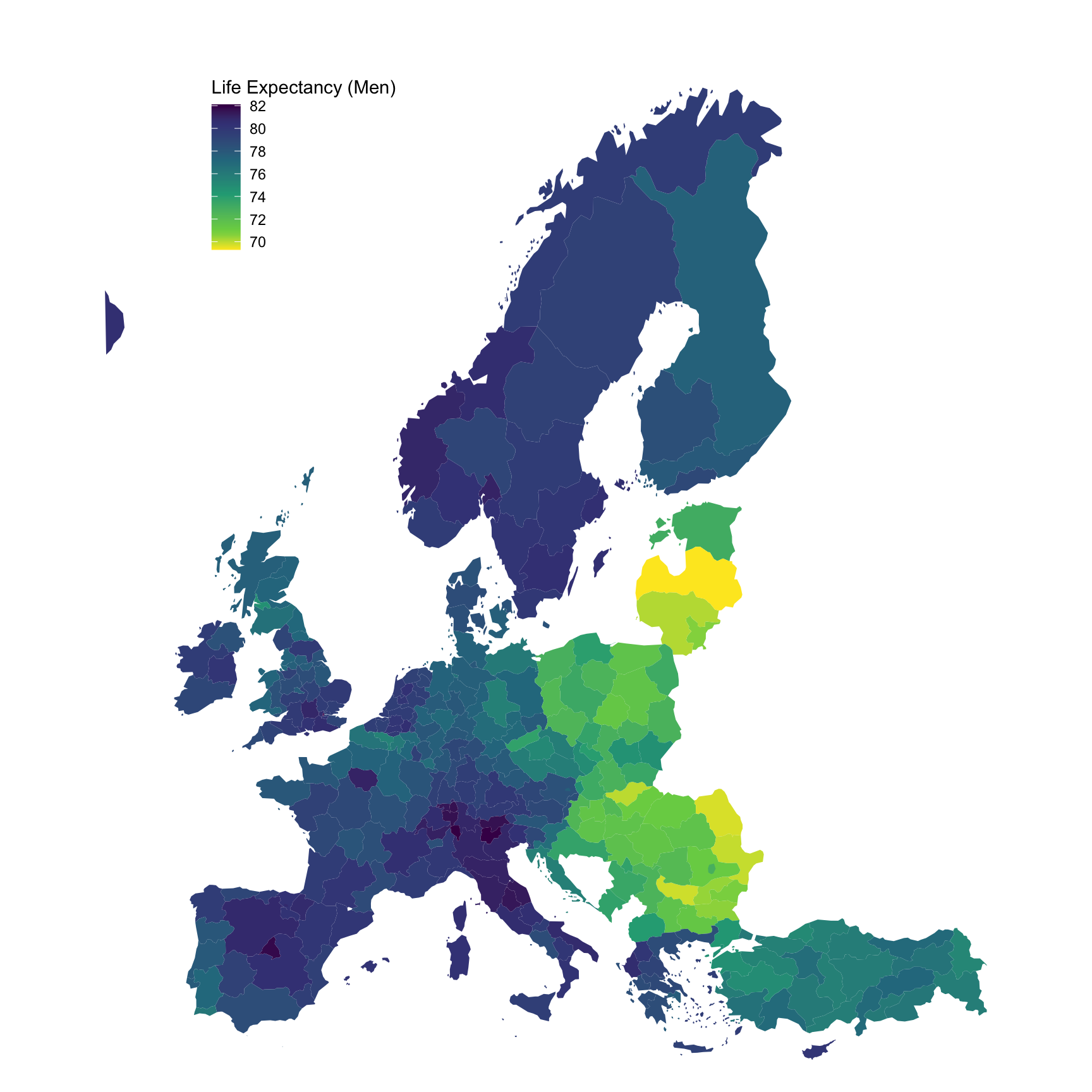

Women

Code

demo_r_mlifexp %>%
  filter(time == "2018", 
         nchar(geo) == 4,
         sex == "F",
         age == "Y1") %>%
  left_join(geo, by = "geo") %>%
  select(geo, Geo, values) %>%
  right_join(europe_NUTS2, by = "geo") %>%
  filter(long >= -15, lat >= 33) %>%
  ggplot(., aes(x = long, y = lat, group = group, fill = values)) +
  geom_polygon() + coord_map() +
  scale_fill_viridis_c(na.value = "white",
                       direction = -1,
                       breaks = seq(70, 90, 2),
                       values = c(0, 0.1, 0.3, 0.5, 0.7, 0.9, 1)) +
  theme_void() + theme(legend.position = c(0.25, 0.85)) + 
  labs(fill = "Life Expectancy (Women)")