Fertility indicators by NUTS 3 region - demo_r_find3

Data - Eurostat

Info

Last observation: Annual: 2024 (N = 4,882)

First observation: Annual: 2013 (N = 3,472)

Last data update: 23 jul 2026, 23:02. Last compile: 24 jul 2026, 01:06

Structure

freq

indic_de

unit

geo

Mean Age at Birth (AGEMOTH)

Table

demo_r_find3 %>%
  filter(indic_de == "AGEMOTH", 
         nchar(geo) == 5,
         time == "2018") %>%
  
  select(geo, Geo, values) %>%
  {if (is_html_output()) datatable(., filter = 'top', rownames = F) else .}

Map

demo_r_find3 %>%
  filter(indic_de == "AGEMOTH", 
         nchar(geo) == 5,
         time == "2018") %>%
  select(geo, values) %>%
  
  right_join(europe_NUTS3, by = "geo") %>%
  filter(long >= -15, lat >= 33, values <= 80000) %>%
  ggplot(., aes(x = long, y = lat, group = group, fill = values)) +
  geom_polygon() + coord_map() +
  scale_fill_viridis_c(na.value = "white",
                       labels = scales::dollar_format(accuracy = 1, prefix = "", suffix = ""),
                       breaks = seq(20, 40, 2),
                       direction = -1) +
  theme_void() + theme(legend.position = c(0.25, 0.85)) + 
  labs(fill = "Mean Age of Birth")

Median Age at Birth (MEDAGEMOTH)

Table

demo_r_find3 %>%
  filter(indic_de == "MEDAGEMOTH", 
         nchar(geo) == 5,
         time == "2018") %>%
  
  select(geo, Geo, values) %>%
  {if (is_html_output()) datatable(., filter = 'top', rownames = F) else .}

Map

demo_r_find3 %>%
  filter(indic_de == "MEDAGEMOTH", 
         nchar(geo) == 5,
         time == "2018") %>%
  select(geo, values) %>%
  
  right_join(europe_NUTS3, by = "geo") %>%
  filter(long >= -15, lat >= 33, values <= 80000) %>%
  ggplot(., aes(x = long, y = lat, group = group, fill = values)) +
  geom_polygon() + coord_map() +
  scale_fill_viridis_c(na.value = "white",
                       labels = scales::dollar_format(accuracy = 1, prefix = "", suffix = ""),
                       breaks = seq(20, 40, 2),
                       direction = -1) +
  theme_void() + theme(legend.position = c(0.25, 0.85)) + 
  labs(fill = "Median Age of Birth")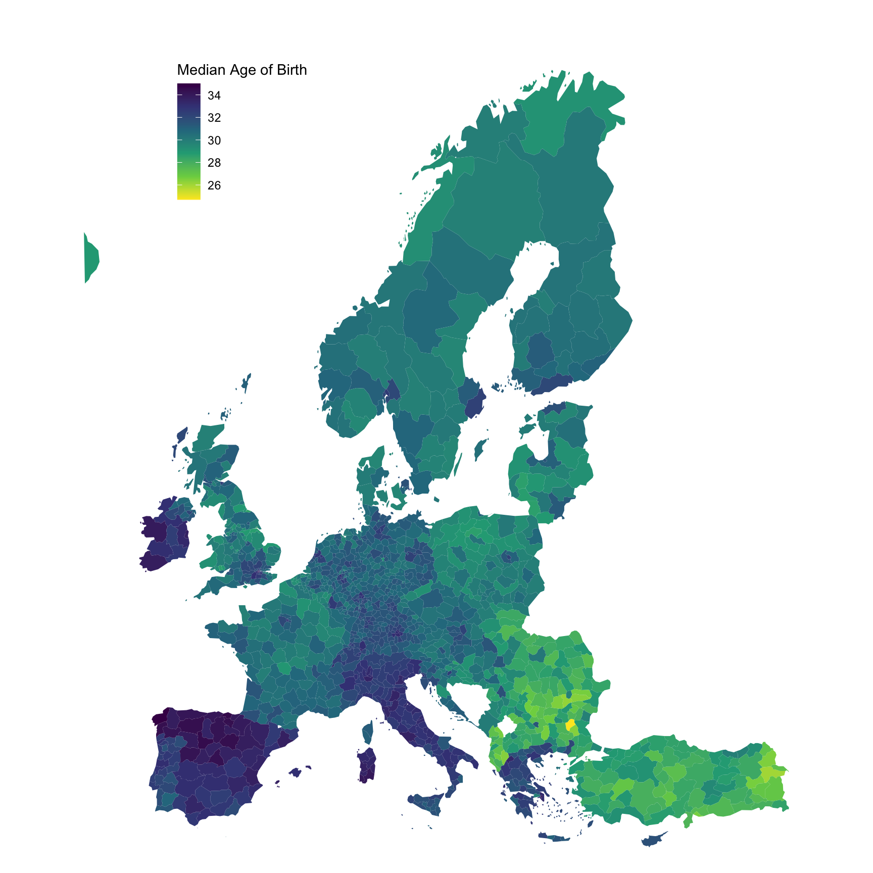

Total fertility rate (TOTFERRT)

Table

demo_r_find3 %>%
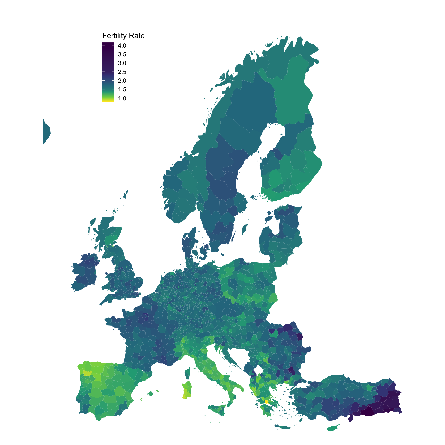
  filter(indic_de == "TOTFERRT", 
         nchar(geo) == 5,
         time == "2018") %>%
  
  select(geo, Geo, values) %>%
  {if (is_html_output()) datatable(., filter = 'top', rownames = F) else .}

Map

demo_r_find3 %>%
  filter(indic_de == "TOTFERRT", 
         nchar(geo) == 5,
         time == "2018") %>%
  select(geo, values) %>%
  
  right_join(europe_NUTS3, by = "geo") %>%
  filter(long >= -15, lat >= 33, values <= 80000) %>%
  ggplot(., aes(x = long, y = lat, group = group, fill = values)) +
  geom_polygon() + coord_map() +
  scale_fill_viridis_c(na.value = "white",
                       labels = scales::dollar_format(accuracy = .1, prefix = "", suffix = ""),
                       values = c(0, 0.05, 0.1, 0.15, 0.2, 0.3, 0.4, 0.5, 1),
                       breaks = seq(0, 4, 0.5),
                       direction = -1) +
  theme_void() + theme(legend.position = c(0.25, 0.85)) + 
  labs(fill = "Fertility Rate")