Population on 1 January by age, sex and NUTS 2 region - demo_r_d2jan

Data - Eurostat

Info

Last observation: Annual: 2025 (N = 137,814)

First observation: Annual: 1990 (N = 84,511)

Last data update: 23 jul 2026, 23:18. Last compile: 24 jul 2026, 01:05

Structure

freq

unit

sex

age

geo

France, Germany, Spain, Italy, Portugal

Total Population

demo_r_d2jan %>%
  filter(geo %in% c("FR", "DE", "ES", "IT", "PT"),
         age == "TOTAL",
         sex == "T") %>%
  year_to_date %>%
  mutate(values = values/1e6) %>%
  left_join(colors, by = c("Geo" = "country")) %>%
  ggplot + geom_line(aes(x = date, y = values, color = color)) +
  theme_minimal() + scale_color_identity() + add_5flags +
  scale_x_date(breaks = as.Date(paste0(seq(1990, 2100, 2), "-01-01")),
               labels = date_format("%Y")) +
  xlab("") + ylab("Population (Millions)")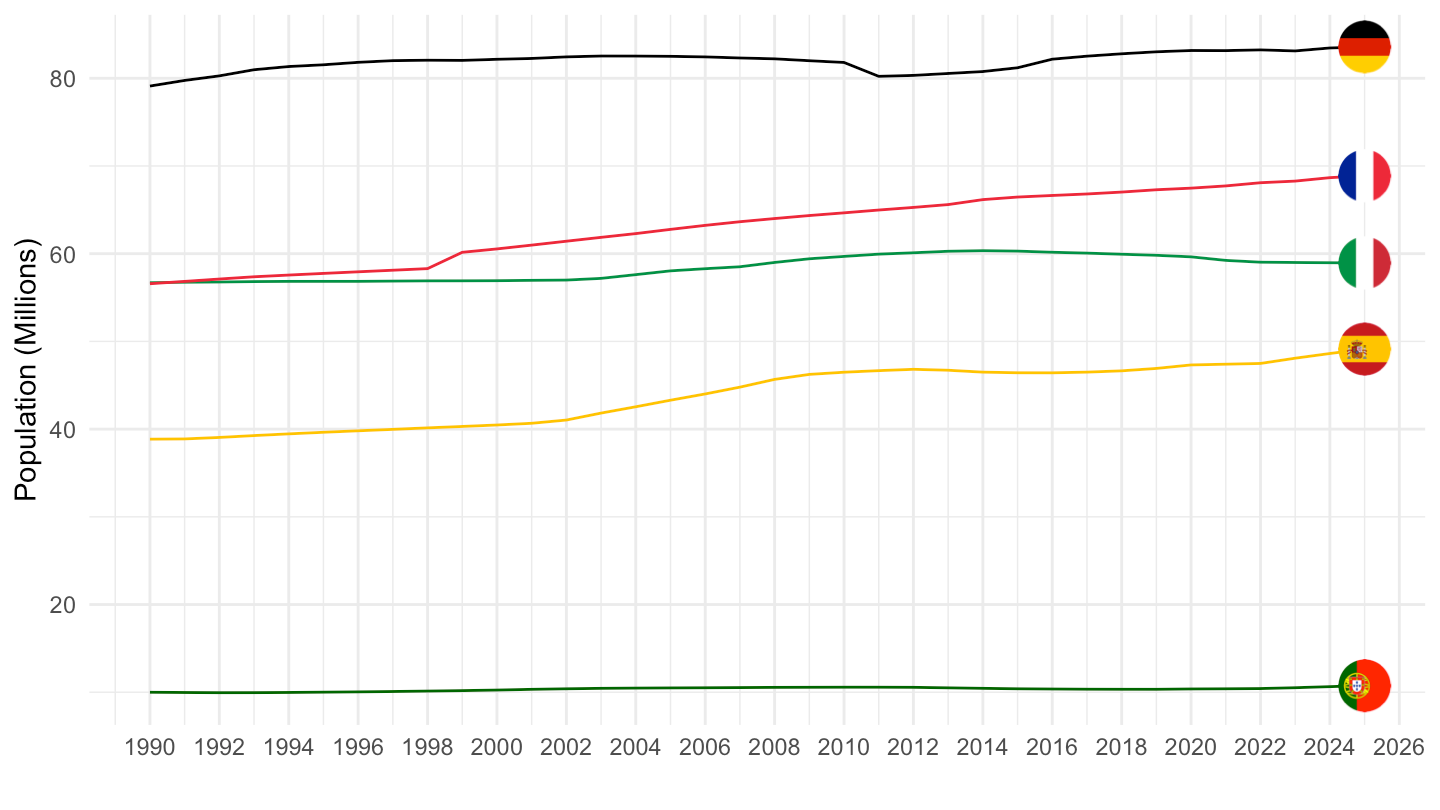

Share of Population Aged 65+

old_ages <- c(paste0("Y", 65:99), "Y_OPEN")

old_pop <- demo_r_d2jan %>%
  filter(geo %in% c("FR", "DE"),
         sex == "T",
         age %in% old_ages,
         !is.na(values)) %>%
  group_by(geo, Geo, time) %>%
  summarise(old = sum(values), .groups = "drop")

demo_r_d2jan %>%
  filter(geo %in% c("FR", "DE"),
         sex == "T",
         age == "TOTAL") %>%
  select(geo, time, total = values) %>%
  left_join(old_pop, ., by = c("geo", "time")) %>%
  mutate(values = old/total) %>%
  year_to_date %>%
  left_join(colors, by = c("Geo" = "country")) %>%
  ggplot + geom_line(aes(x = date, y = values, color = color)) +
  theme_minimal() + scale_color_identity() + add_flags +
  scale_x_date(breaks = as.Date(paste0(seq(1990, 2100, 2), "-01-01")),
               labels = date_format("%Y")) +
  xlab("") + ylab("Population aged 65+ (% of total)") +
  scale_y_continuous(labels = scales::percent_format(accuracy = 1))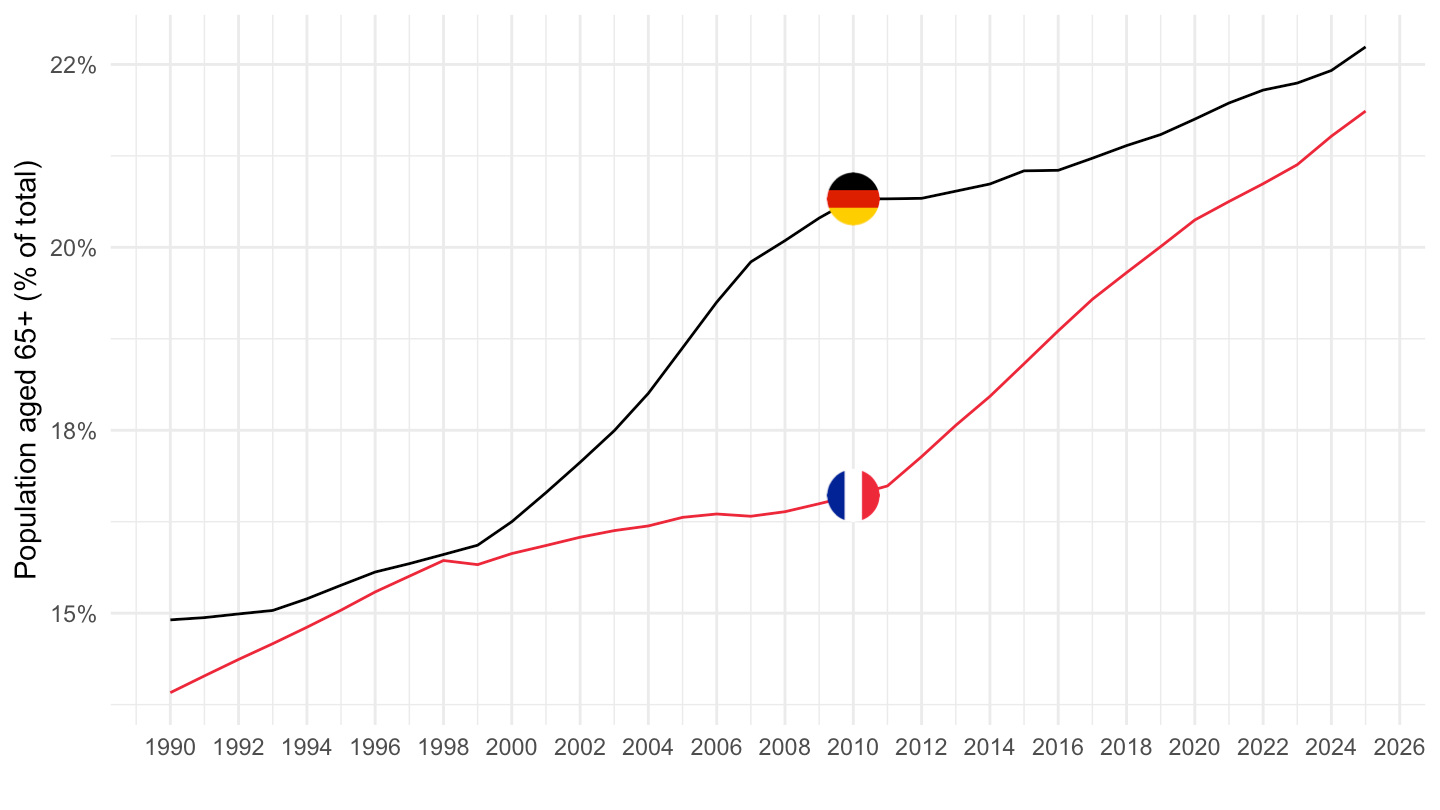

Population

demo_r_d2jan %>%
  filter(nchar(geo) == 4,
         time == "2018",
         sex == "T",
         age == "TOTAL") %>%
  
  select(geo, Geo, values) %>%
  {if (is_html_output()) datatable(., filter = 'top', rownames = F) else .}