Last observation: 2011 (N = 3636204)
First observation: 2011 (N = 3636204)
Last data update: 09 sept. 2026, 08:00
Last compile: 04 oct. 2026, 23:01
cens_11empo_r2 |>
  filter(nchar(geo) == 2,
         age == "TOTAL",
         sex == "T",
         isco08 == "TOTAL",
         wstatus %in% c("EMP", "SELF_S", "SELF_NS")) |>
  select(geo, Geo, wstatus, values) |>
  spread(wstatus, values) |>
  mutate(rate = (SELF_S + SELF_NS) / EMP) |>
  filter(!is.na(rate)) |>
  add_flag_color("Geo") |>
  mutate(color = ifelse(is.na(color), "grey50", color)) |>
  ggplot() + geom_col(aes(x = reorder(Geo, rate), y = rate, fill = color)) +
  scale_fill_identity() +
  coord_flip() +
  theme_minimal() +
  xlab("") + ylab("Self-employed share of employed population, 2011") +
  scale_y_continuous(labels = scales::percent_format(accuracy = 1))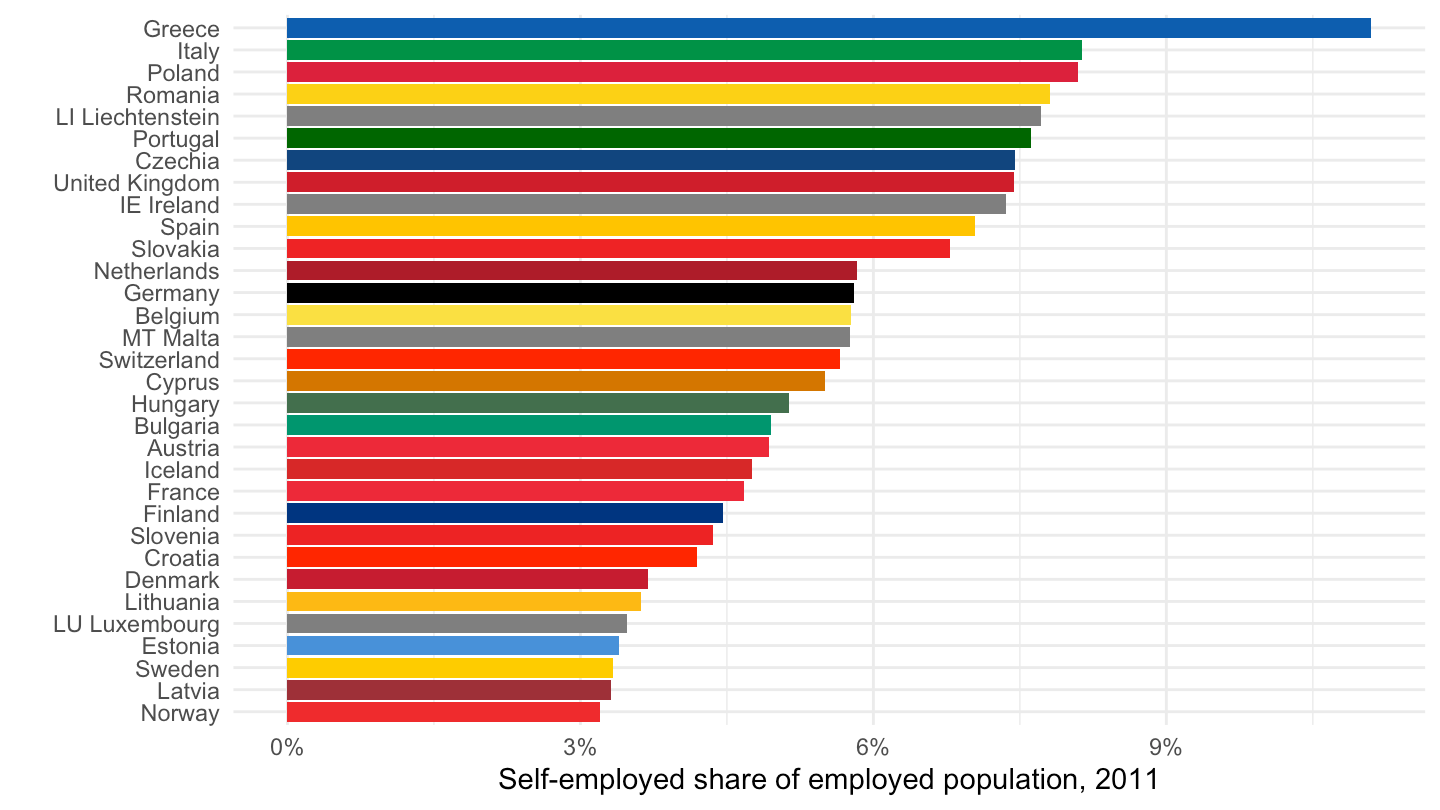
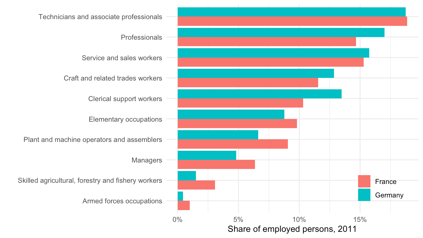
cens_11empo_r2 |>
  filter(geo %in% c("FR", "DE"),
         age == "TOTAL",
         sex == "T",
         wstatus == "EMP",
         !isco08 %in% c("NAP", "TOTAL", "UNK")) |>
  group_by(geo) |>
  mutate(share = values / sum(values)) |>
  ungroup() |>
  ggplot() + geom_col(aes(x = reorder(Isco08, share), y = share, fill = Geo),
                     position = "dodge") +
  coord_flip() +
  theme_minimal() +
  theme(legend.position = c(0.85, 0.12),
        legend.title = element_blank()) +
  xlab("") + ylab("Share of employed persons, 2011") +
  scale_y_continuous(labels = scales::percent_format(accuracy = 1))