Total and active population by sex, age, employment status, residence one year prior to the census and NUTS 3 regions - cens_01rapop

Data - Eurostat

Info

Last observation: Annual: 2001 (N = 558,223)

First observation: Annual: 2001 (N = 558,223)

Last data update: 11 aoû 2026, 22:31. Last compile: 11 aoû 2026, 23:16

Structure

freq

wstatus

age

sex

unit

geo

Country Comparison, 2001

Unemployment Rate (Active Population)

cens_01rapop |>
  filter(nchar(geo) == 2,
         wstatus %in% c("ACT", "UNE"),
         age == "TOTAL",
         sex == "T") |>
  select(Geo, wstatus, values) |>
  spread(wstatus, values) |>
  mutate(urate = UNE/ACT) |>
  ggplot() + geom_col(aes(x = reorder(Geo, urate), y = urate), fill = "steelblue") +
  coord_flip() +
  theme_minimal() +
  xlab("") + ylab("Unemployment rate (2001 census, % of active population)") +
  scale_y_continuous(labels = scales::percent_format(accuracy = 1))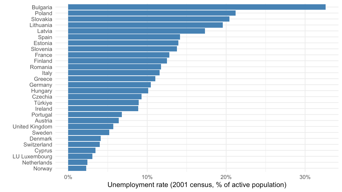

France: Labour Force Status by Age, 2001

Employed, Unemployed, Inactive

cens_01rapop |>
  filter(geo == "FR",
         wstatus %in% c("EMP", "UNE", "INAC"),
         !age %in% c("TOTAL", "UNK"),
         sex == "T") |>
  ggplot() + geom_col(aes(x = Age, y = values/1e6, fill = Wstatus)) +
  theme_minimal() +
  theme(axis.text.x = element_text(angle = 45, hjust = 1),
        legend.position = c(0.8, 0.8),
        legend.title = element_blank()) +
  xlab("") + ylab("Persons (Millions)")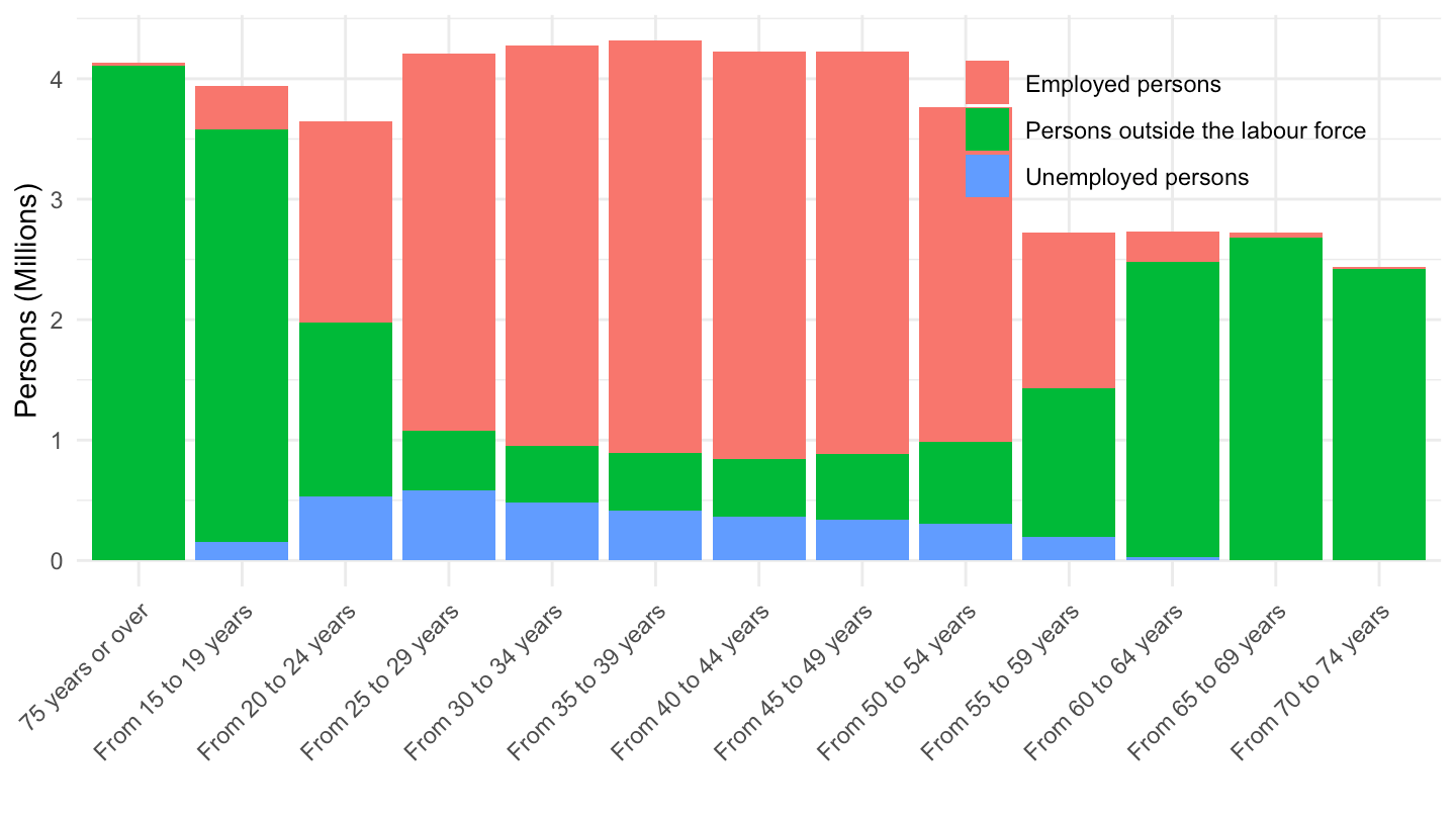

Latest Census by Country

cens_01rapop |>
  filter(nchar(geo) == 2,
         wstatus %in% c("POP", "ACT", "EMP", "UNE"),
         age == "TOTAL",
         sex == "T") |>
  mutate(values = values/1e6) |>
  select(Geo, wstatus, values) |>
  spread(wstatus, values) |>
  mutate(urate = round(100*UNE/ACT, 1)) |>
  arrange(-POP) |>
  print_table_conditional()

Geo	ACT	EMP	POP	UNE	urate
Türkiye	28.544359	25.997141	67.803927	2.547218	8.9
Italy	23.742262	20.993732	56.995744	2.748530	11.6
United Kingdom	28.185423	26.575681	56.960066	1.609742	5.7
France	26.535140	23.048776	47.440481	3.400749	12.8
Spain	19.030918	16.338142	40.595861	2.692776	14.1
Poland	16.776498	13.218344	38.230080	3.558154	21.2
Germany	34.714606	31.088487	34.714606	3.626119	10.4
Romania	8.851831	7.811733	21.680974	1.040098	11.8
Netherlands	7.586914	7.394777	15.985538	0.182777	2.4
Greece	4.610129	4.101949	10.934097	0.508180	11.0
Portugal	4.990208	4.650947	10.356117	0.339261	6.8
Czechia	5.253400	4.766463	10.230060	0.486937	9.3
Hungary	4.106479	3.690269	10.198315	0.416210	10.1
Sweden	4.285541	4.062965	8.882792	0.222576	5.2
Austria	3.986761	3.731544	8.032926	0.255217	6.4
Bulgaria	3.854993	2.598024	7.928901	1.256969	32.6
Switzerland	3.946988	3.789416	7.288010	0.157572	4.0
Slovakia	2.748050	2.186836	5.379455	0.561214	20.4
Denmark	2.874552	2.756032	5.349212	0.118520	4.1
Finland	2.546661	2.228557	5.181115	0.318104	12.5
Norway	2.326397	2.273744	4.520947	0.052653	2.3
Ireland	1.767645	1.610881	3.858495	0.156764	8.9
Lithuania	1.576572	1.268195	3.483972	0.308377	19.6
Latvia	1.020955	0.844262	2.377383	0.176693	17.3
Slovenia	0.949078	0.818304	1.964036	0.130774	13.8
Estonia	0.632849	0.544650	1.370052	0.088199	13.9
Cyprus	0.303198	0.292732	0.542087	0.010466	3.5
LU Luxembourg	0.191181	0.185352	0.439539	0.005829	3.0

2001 Unemployed

cens_01rapop |>
  filter(nchar(geo) == 5,
         wstatus %in% c("ACT", "UNE"),
         age == "TOTAL",
         sex == "T") |>
  select(geo, wstatus, values) |>
  spread(wstatus, values) |>
  
  right_join(europe_NUTS3, by = "geo") |>
  filter(long >= -15, lat >= 33) |>
  ggplot(aes(x = long, y = lat, group = group, fill = UNE/ACT)) +
  geom_polygon() + coord_map() +
  scale_fill_viridis_c(na.value = "white",
                       direction = -1,
                       labels = percent_format(accuracy = 1),
                       breaks = 0.01*seq(0, 90, 5),
                       values = c(0, 0.1, 0.2, 0.3, 0.4, 0.5, 1)) +
  theme_void() + theme(legend.position = c(0.25, 0.85)) + 
  labs(fill = "Manuf Share")