Total and active population by sex, age, employment status, residence one year prior to the census and NUTS 3 regions - cens_01ramigr

Data - Eurostat

Author

François Geerolf

Info

Last observation: Annual: 2001 (N = 1,485,361)

First observation: Annual: 2001 (N = 1,485,361)

Last data update: 23 jul 2026, 22:29. Last compile: 24 jul 2026, 00:58

Structure

Migration in the Year Before the Census

This dataset is a single cross-section (census reference year), so the charts below compare countries and age groups rather than tracking a time series.

By Country

Code

latest_t <- cens_01ramigr %>%
  filter(!is.na(values)) %>%
  summarise(m = max(time)) %>%
  pull(m)

cens_01ramigr %>%
  filter(time == latest_t,
         nchar(geo) == 2,
         sex == "T",
         age == "TOTAL",
         wstatus == "POP",
         resid %in% c("CHG_OUT", "TOTAL")) %>%
  select(geo, Geo, resid, values) %>%
  spread(resid, values) %>%
  filter(!is.na(CHG_OUT), !is.na(TOTAL)) %>%
  mutate(rate = CHG_OUT / TOTAL) %>%
  arrange(rate) %>%
  mutate(Geo = factor(Geo, levels = Geo)) %>%
  ggplot + geom_col(aes(x = Geo, y = rate), fill = "steelblue") +
  coord_flip() +
  theme_minimal() +
  xlab("") + ylab("Share of population resident outside the country one year earlier") +
  scale_y_continuous(labels = scales::percent_format(accuracy = 0.1))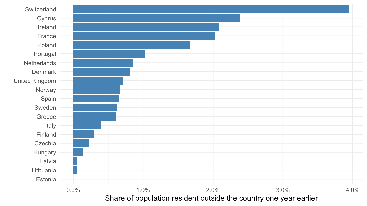

Age Profile: Poland

Code

age_bands <- c("Y5-9", "Y10-14", "Y15-19", "Y20-24", "Y25-29", "Y30-34", "Y35-39",
               "Y40-44", "Y45-49", "Y50-54", "Y55-59", "Y60-64", "Y65-69", "Y70-74",
               "Y75-79", "Y80-84", "Y85-89", "Y90-94", "Y95-99")

cens_01ramigr %>%
  filter(time == latest_t,
         geo == "PL",
         sex == "T",
         wstatus == "POP",
         age %in% age_bands,
         resid %in% c("CHG_OUT", "TOTAL")) %>%
  select(age, resid, values) %>%
  spread(resid, values) %>%
  mutate(rate = CHG_OUT / TOTAL,
         age = factor(age, levels = age_bands)) %>%
  ggplot + geom_col(aes(x = age, y = rate), fill = "darkred") +
  theme_minimal() +
  theme(axis.text.x = element_text(angle = 45, hjust = 1)) +
  xlab("") + ylab("Share who changed residence from outside Poland (past year)") +
  scale_y_continuous(labels = scales::percent_format(accuracy = 0.1))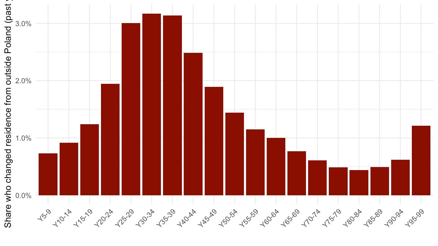

Snapshot by Country

Code

cens_01ramigr %>%
  filter(time == latest_t,
         nchar(geo) == 2,
         sex == "T",
         age == "TOTAL",
         wstatus == "POP",
         resid %in% c("CHG_OUT", "CHG_OUT3", "TOTAL")) %>%
  select(Geo, resid, values) %>%
  spread(resid, values) %>%
  mutate(`Rate (CHG_OUT/TOTAL)` = scales::percent(CHG_OUT / TOTAL, accuracy = 0.1)) %>%
  arrange(desc(CHG_OUT)) %>%
  print_table_conditional()

Geo	CHG_OUT	CHG_OUT3	TOTAL	Rate (CHG_OUT/TOTAL)
France	1187182	8896369	58513700	2.0%
Poland	633595	748104	37878418	1.7%
United Kingdom	406706	2036178	57733848	0.7%
Switzerland	288003	388604	7288010	4.0%
Spain	265692	209100	40847371	0.7%
Italy	223634	706717	56995744	0.4%
Netherlands	137013	313555	15985538	0.9%
Portugal	105705	120195	10356117	1.0%
Greece	67251	218721	10934097	0.6%
Ireland	64605	52316	3106824	2.1%
Sweden	55961	167088	8882792	0.6%
Denmark	43663	148201	5349212	0.8%
Norway	30380	100412	4520947	0.7%
Czechia	22805	56483	10230060	0.2%
Cyprus	16471	NA	689565	2.4%
Finland	15283	103800	5181115	0.3%
Hungary	14388	103668	10198315	0.1%
Lithuania	1661	0	3483972	0.0%
Latvia	1275	7639	2377383	0.1%
Estonia	0	0	1370052	0.0%
Austria	NA	NA	8032926	NA
Germany	NA	NA	82259540	NA
LU Luxembourg	NA	NA	439539	NA
Slovakia	NA	NA	5379455	NA
Slovenia	NA	7192	1964036	NA