| LAST_COMPILE |
|---|
| 2026-07-24 |
Indices of Consumer prices - ICP
Data - ECB
Info
LAST_COMPILE
Last
| TIME_PERIOD | FREQ | Nobs |
|---|---|---|
| 2025-Q4 | Q | 963 |
| 2025-12 | M | 24836 |
| 2025 | A | 26052 |
Nobs
ICP_ITEM
Code
ICP %>%
  left_join(ICP_ITEM,  by = "ICP_ITEM") %>%
  group_by(ICP_ITEM, Icp_item) %>%
  summarise(Nobs = n()) %>%
  arrange(-Nobs) %>%
  {if (is_html_output()) datatable(., filter = 'top', rownames = F) else .}
ICP_SUFFIX
Code
ICP %>%
  left_join(ICP_SUFFIX,  by = "ICP_SUFFIX") %>%
  group_by(ICP_SUFFIX, Icp_suffix) %>%
  summarise(Nobs = n()) %>%
  arrange(-Nobs) %>%
{if (is_html_output()) print_table(.) else .}| ICP_SUFFIX | Icp_suffix | Nobs |
|---|---|---|
| INX | Index | 3088906 |
| ANR | Annual rate of change | 2934228 |
| INW | Sub-index weight | 285019 |
| AVR | Annual average rate of change | 243731 |
| CTG | Contribution to growth rate | 55560 |
| QUR | Quarterly rate of change | 22503 |
| OHW | OOHPI weight (all OOHPI items = 1000) | 6366 |
| D0W | EU (changing composition) country weights | 5412 |
| V5W | EU 27 (as of brexit) country weights | 4882 |
| U2W | Euro area country weights | 3837 |
| I9W | NA | 3546 |
| I8W | Euro 19 country weights | 3344 |
| V3W | EU 28 country weights | 3211 |
| 3MM | Three-month moving average | 1169 |
| MOR | Monthly rate of change | 347 |
| CTR | Annual rate of change at constant tax rates (HICP-CT) | 37 |
UNIT
Code
ICP %>%
  group_by(UNIT) %>%
  summarise(Nobs = n()) %>%
  arrange(-Nobs) %>%
{if (is_html_output()) print_table(.) else .}| UNIT | Nobs |
|---|---|
| PURE_NUMB | 3375374 |
| PCCH | 3198357 |
| PD | 55272 |
| IX | 32807 |
| POINTS | 288 |
TITLE
Code
ICP %>%
  group_by(TITLE) %>%
  summarise(Nobs = n()) %>%
  arrange(-Nobs) %>%
  {if (is_html_output()) datatable(., filter = 'top', rownames = F) else .}
FREQ
Code
ICP %>%
  left_join(FREQ,  by = "FREQ") %>%
  group_by(FREQ, Freq) %>%
  summarise(Nobs = n()) %>%
  arrange(-Nobs) %>%
{if (is_html_output()) print_table(.) else .}| FREQ | Freq | Nobs |
|---|---|---|
| M | Monthly | 6029946 |
| A | Annual | 565080 |
| Q | Quarterly | 67072 |
UNIT
Code
ICP %>%
  left_join(UNIT,  by = "UNIT") %>%
  group_by(UNIT, Unit) %>%
  summarise(Nobs = n()) %>%
  arrange(-Nobs) %>%
{if (is_html_output()) print_table(.) else .}| UNIT | Unit | Nobs |
|---|---|---|
| PURE_NUMB | Pure number | 3375374 |
| PCCH | Percentage change | 3198357 |
| PD | Percentage points | 55272 |
| IX | Index | 32807 |
| POINTS | Points | 288 |
STS_INSTITUTION
Code
ICP %>%
  mutate(STS_INSTITUTION = paste0(STS_INSTITUTION)) %>%
  left_join(STS_INSTITUTION,  by = "STS_INSTITUTION") %>%
  group_by(STS_INSTITUTION, Sts_institution) %>%
  summarise(Nobs = n()) %>%
  arrange(-Nobs) %>%
  {if (is_html_output()) datatable(., filter = 'top', rownames = F) else .}
REF_AREA
Code
ICP %>%
  left_join(REF_AREA,  by = "REF_AREA") %>%
  group_by(REF_AREA, Ref_area) %>%
  summarise(Nobs = n()) %>%
  arrange(-Nobs) %>%
  {if (is_html_output()) datatable(., filter = 'top', rownames = F) else .}
ADJUSTMENT
Code
ICP %>%
  left_join(ADJUSTMENT,  by = "ADJUSTMENT") %>%
  group_by(ADJUSTMENT, Adjustment) %>%
  summarise(Nobs = n()) %>%
  arrange(-Nobs) %>%
  {if (is_html_output()) datatable(., filter = 'top', rownames = F) else .}
UNIT_INDEX_BASE
Code
ICP %>%
  group_by(UNIT_INDEX_BASE) %>%
  summarise(Nobs = n()) %>%
  arrange(-Nobs) %>%
{if (is_html_output()) print_table(.) else .}| UNIT_INDEX_BASE | Nobs |
|---|---|
| 3279100 | |
| 2015 = 100 | 2967104 |
| Parts per 1000. HICP total = 1000 | 284843 |
| 2005 = 100 | 121802 |
| Parts per 1000. EU total = 1000 | 5412 |
| Parts per 1000. EMU total = 1000 | 3837 |
DECIMALS
Code
ICP %>%
  group_by(DECIMALS) %>%
  summarise(Nobs = n()) %>%
  arrange(-Nobs) %>%
{if (is_html_output()) print_table(.) else .}| DECIMALS | Nobs |
|---|---|
| 1 | 3870627 |
| 2 | 2790580 |
| 6 | 891 |
TIME_FORMAT
Code
ICP %>%
  group_by(TIME_FORMAT) %>%
  summarise(Nobs = n()) %>%
  arrange(-Nobs) %>%
{if (is_html_output()) print_table(.) else .}| TIME_FORMAT | Nobs |
|---|---|
| P1M | 6029946 |
| P1Y | 565080 |
| P3M | 67072 |
Info
Housing
Greece
Code
ICP %>%
  filter(REF_AREA %in% c("GR"),
         ICP_ITEM %in% c("HOUSE0", "041000", "040000"),
         ICP_SUFFIX == "INX") %>%
  left_join(ICP_ITEM, by = "ICP_ITEM") %>%
  month_to_date() %>%
  filter(!is.na(OBS_VALUE)) %>%
  ggplot() +  ylab("HICP - Overall index") + xlab("") + theme_minimal() +
  geom_line(aes(x = date, y = OBS_VALUE, color = Icp_item)) +

  theme(legend.position = c(0.65, 0.15),
        legend.title = element_blank()) +
  scale_x_date(breaks = seq(1920, 2100, 2) %>% paste0("-01-01") %>% as.Date,
               labels = date_format("%Y")) +
  scale_y_log10(breaks = seq(0, 200, 5),
                     labels = dollar_format(accuracy = 1, prefix = ""))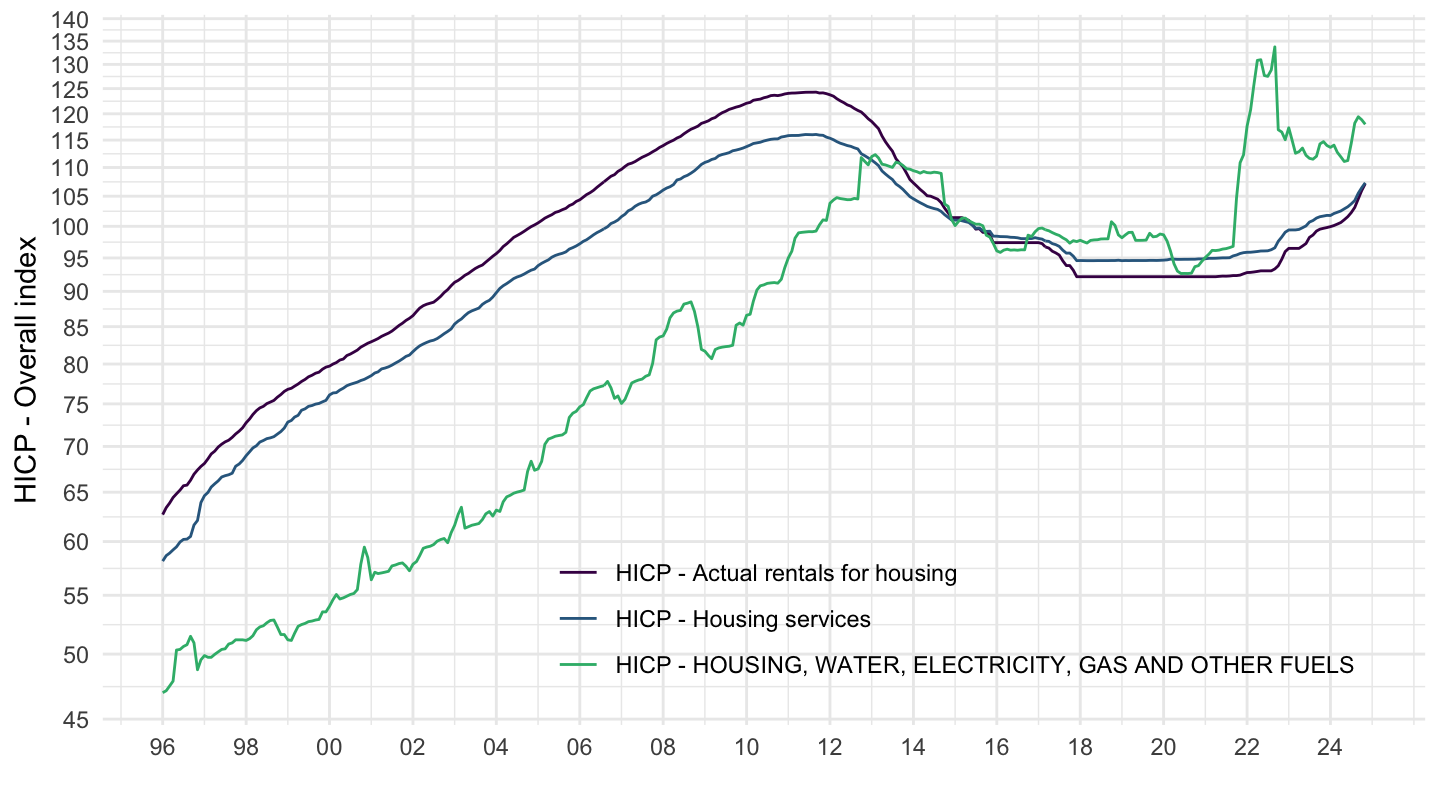
Spain
Code
ICP %>%
  filter(REF_AREA %in% c("ES"),
         ICP_ITEM %in% c("HOUSE0", "041000", "040000"),
         ICP_SUFFIX == "INX") %>%
  left_join(ICP_ITEM, by = "ICP_ITEM") %>%
  month_to_date() %>%
  filter(!is.na(OBS_VALUE)) %>%
  ggplot() +  ylab("HICP - Overall index") + xlab("") + theme_minimal() +
  geom_line(aes(x = date, y = OBS_VALUE, color = Icp_item)) +

  theme(legend.position = c(0.65, 0.15),
        legend.title = element_blank()) +
  scale_x_date(breaks = seq(1920, 2100, 2) %>% paste0("-01-01") %>% as.Date,
               labels = date_format("%Y")) +
  scale_y_log10(breaks = seq(0, 200, 5),
                     labels = dollar_format(accuracy = 1, prefix = ""))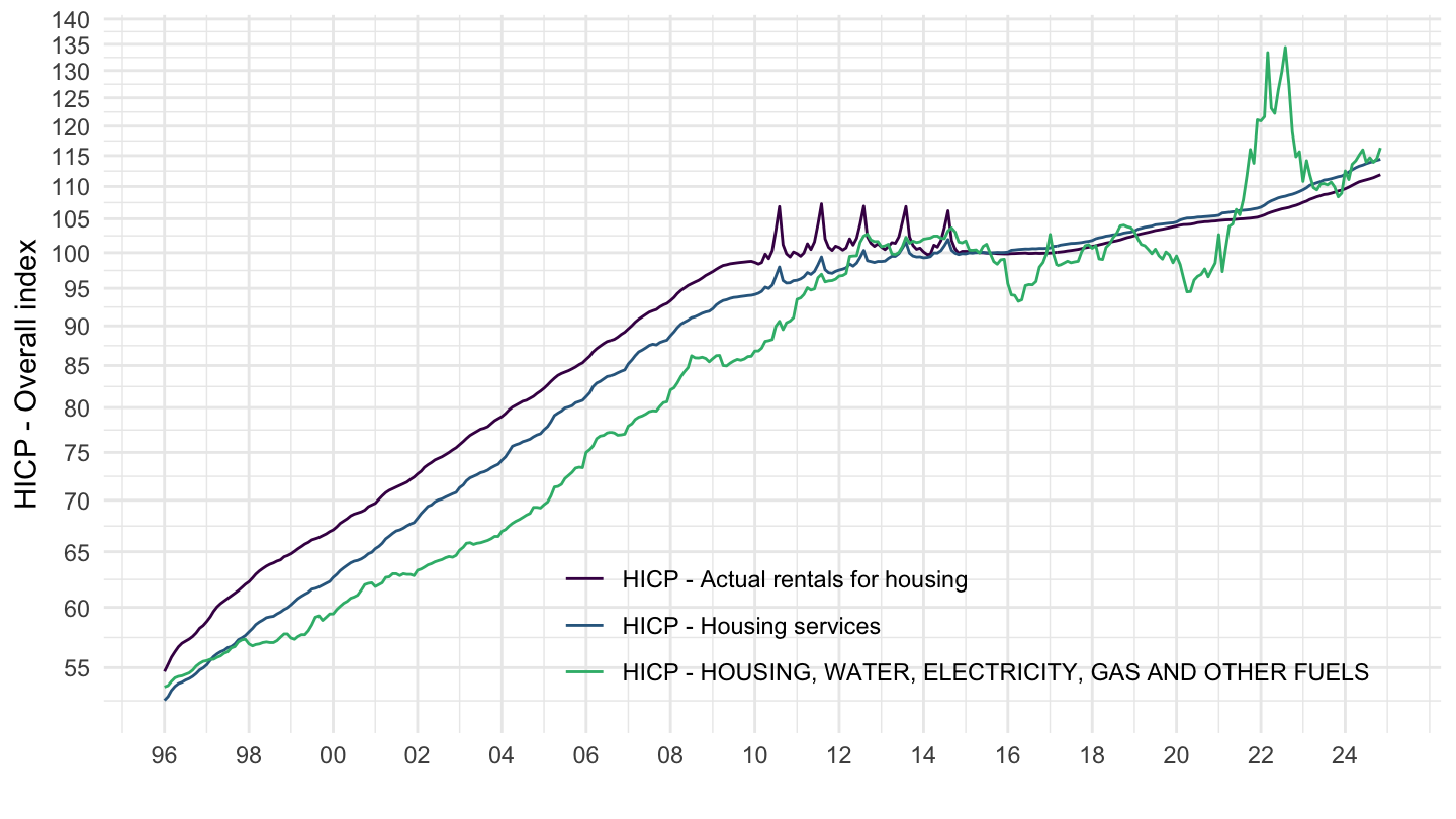
France
Code
ICP %>%
  filter(REF_AREA %in% c("FR"),
         ICP_ITEM %in% c("HOUSE0", "041000", "040000"),
         ICP_SUFFIX == "INX") %>%
  left_join(ICP_ITEM, by = "ICP_ITEM") %>%
  month_to_date() %>%
  filter(!is.na(OBS_VALUE)) %>%
  ggplot() +  ylab("HICP - Overall index") + xlab("") + theme_minimal() +
  geom_line(aes(x = date, y = OBS_VALUE, color = Icp_item)) +

  theme(legend.position = c(0.65, 0.15),
        legend.title = element_blank()) +
  scale_x_date(breaks = seq(1920, 2100, 2) %>% paste0("-01-01") %>% as.Date,
               labels = date_format("%Y")) +
  scale_y_log10(breaks = seq(0, 200, 5),
                     labels = dollar_format(accuracy = 1, prefix = ""))
Harmonised Index of Consumer Prices - HICP
Euro area Broad Indexes (1960-)
Code
ICP %>%
  filter(REF_AREA %in% c("U2"),
         # 000000: HICP - Overall index
         # XEF000: HICP - All-items excluding energy and food
         ICP_ITEM %in% c("000000", "XEF000", "XE0000"),
         # ANR: Annual Rate of Change
         ICP_SUFFIX == "ANR",
         FREQ == "M") %>%
  left_join(REF_AREA,  by = "REF_AREA") %>%
  month_to_date() %>%
  filter(!is.na(OBS_VALUE)) %>%
  ggplot() + theme_minimal() + ylab("HICP - Broad indexes") + xlab("") +
  geom_line(aes(x = date, y = OBS_VALUE/100, color = TITLE)) +

  scale_x_date(breaks = seq(1920, 2100, 2) %>% paste0("-01-01") %>% as.Date,
               labels = date_format("%Y")) +
  theme(legend.position = c(0.75, 0.9),
        legend.title = element_blank()) +
  scale_y_continuous(breaks = 0.01*seq(0, 200, 1),
                labels = percent_format(accuracy = 1))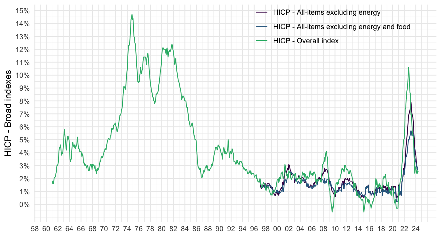
Euro area Broad Indexes (1996-)
Code
ICP %>%
  filter(REF_AREA %in% c("U2"),
         # 000000: HICP - Overall index
         # XEF000: HICP - All-items excluding energy and food
         ICP_ITEM %in% c("000000", "XEF000", "XE0000"),
         # ANR: Annual Rate of Change
         ICP_SUFFIX == "ANR",
         FREQ == "M") %>%
  left_join(REF_AREA,  by = "REF_AREA") %>%
  month_to_date() %>%
  filter(!is.na(OBS_VALUE),
         date >= as.Date("1996-01-01")) %>%
  ggplot() + theme_minimal() + ylab("HICP - Broad indexes") + xlab("") +
  geom_line(aes(x = date, y = OBS_VALUE/100, color = TITLE)) +
  scale_x_date(breaks = seq(1920, 2100, 2) %>% paste0("-01-01") %>% as.Date,
               labels = date_format("%Y")) +
  theme(legend.position = c(0.75, 0.9),
        legend.title = element_blank()) +
  scale_y_continuous(breaks = 0.01*seq(0, 200, 1),
                labels = percent_format(accuracy = 1))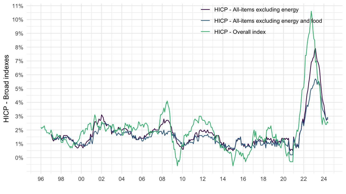
Euro area Broad Indexes (2008-)
Code
ICP %>%
  filter(REF_AREA %in% c("U2"),
         # 000000: HICP - Overall index
         # XEF000: HICP - All-items excluding energy and food
         ICP_ITEM %in% c("000000", "XEF000", "XE0000"),
         # ANR: Annual Rate of Change
         ICP_SUFFIX == "ANR",
         FREQ == "M") %>%
  left_join(REF_AREA,  by = "REF_AREA") %>%
  month_to_date() %>%
  filter(!is.na(OBS_VALUE),
         date >= as.Date("2007-01-01")) %>%
  ggplot() + theme_minimal() + ylab("HICP - Broad indexes") + xlab("") +
  geom_line(aes(x = date, y = OBS_VALUE/100, color = KEY)) +
  scale_x_date(breaks = seq(1920, 2100, 2) %>% paste0("-01-01") %>% as.Date,
               labels = date_format("%Y")) +
  theme(legend.position = c(0.75, 0.9),
        legend.title = element_blank()) +
  scale_y_continuous(breaks = 0.01*seq(0, 200, 1),
                labels = percent_format(accuracy = 1))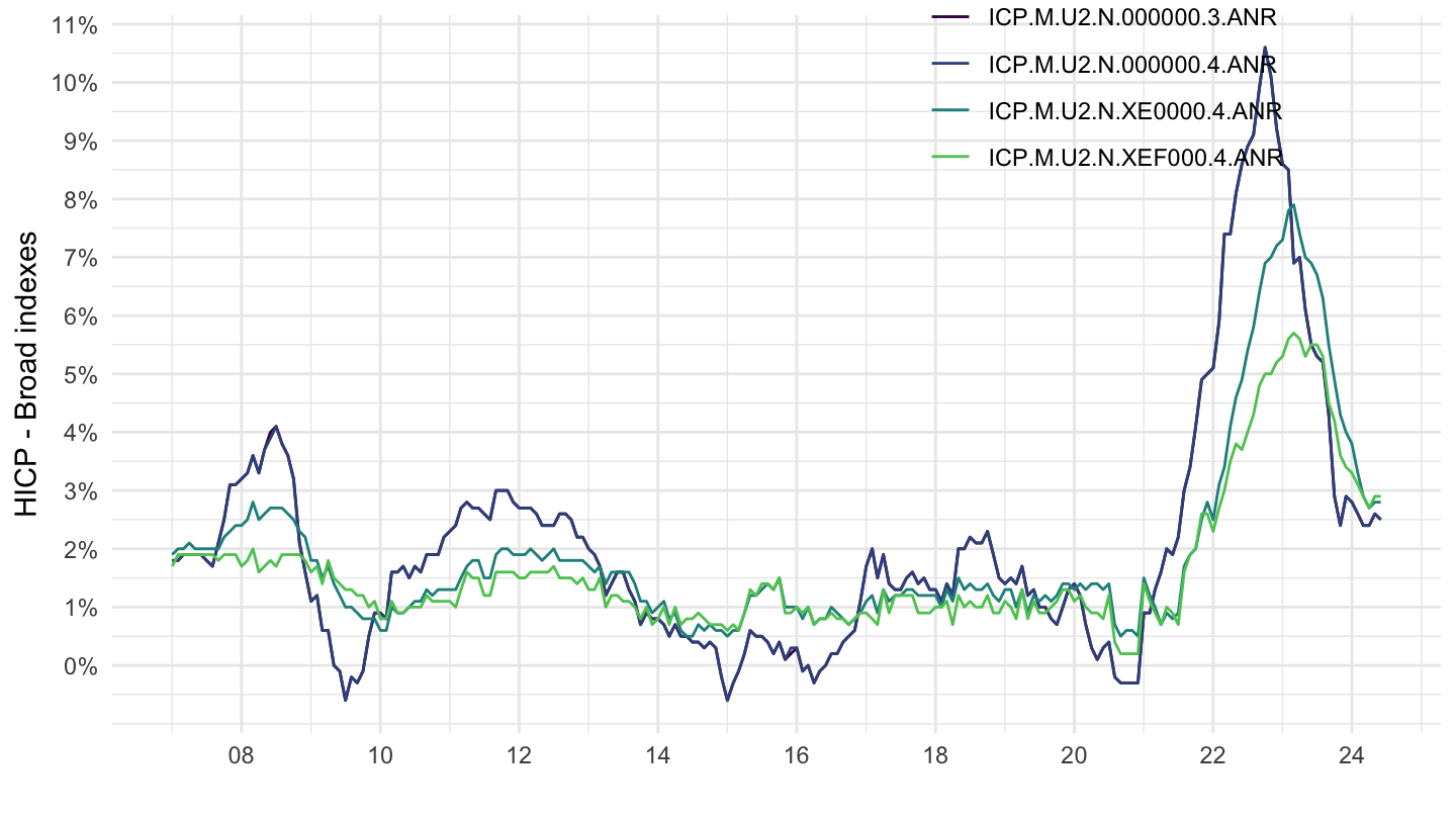
Spain Broad Indexes
1996-2021
Code
ICP %>%
  filter(REF_AREA %in% c("ES"),
         # 000000: HICP - Overall index
         # XEF000: HICP - All-items excluding energy and food
         ICP_ITEM %in% c("000000", "XEF000", "XE0000"),
         # ANR: Annual Rate of Change
         ICP_SUFFIX == "ANR",
         FREQ == "M") %>%
  left_join(REF_AREA,  by = "REF_AREA") %>%
  month_to_date() %>%
  filter(!is.na(OBS_VALUE),
         date >= as.Date("1996-01-01")) %>%
  ggplot() + theme_minimal() + ylab("HICP - Broad indexes") + xlab("") +
  geom_line(aes(x = date, y = OBS_VALUE/100, color = TITLE)) +

  geom_hline(yintercept = 0.02, linetype = "dashed",  color = "black") +
  geom_hline(yintercept = 0, linetype = "dashed",  color = "black") +
  scale_x_date(breaks = seq(1920, 2100, 2) %>% paste0("-01-01") %>% as.Date,
               labels = date_format("%Y")) +
  theme(legend.position = c(0.2, 0.9),
        legend.title = element_blank()) +
  scale_y_continuous(breaks = 0.01*seq(-100, 200, 0.5),
                labels = percent_format(accuracy = 0.1))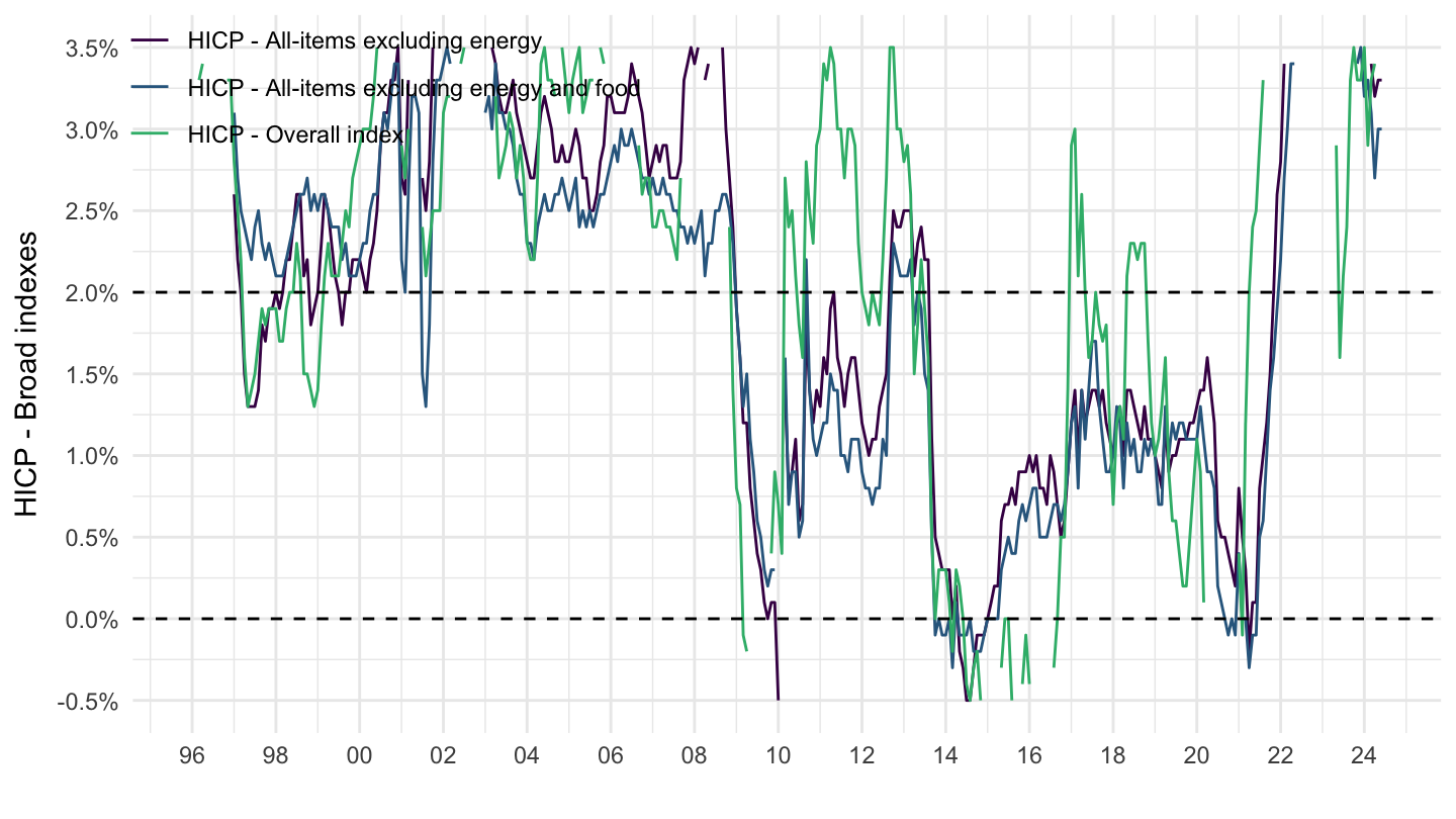
2010-2013
Code
ICP %>%
  filter(REF_AREA %in% c("ES"),
         # 000000: HICP - Overall index
         # XEF000: HICP - All-items excluding energy and food
         ICP_ITEM %in% c("000000", "XEF000", "XE0000"),
         # ANR: Annual Rate of Change
         ICP_SUFFIX == "ANR",
         FREQ == "M") %>%
  left_join(REF_AREA,  by = "REF_AREA") %>%
  month_to_date() %>%
  filter(!is.na(OBS_VALUE),
         date >= as.Date("2010-01-01"),
         date <= as.Date("2014-01-01")) %>%
  ggplot() + theme_minimal() + ylab("HICP - Broad indexes") + xlab("") +
  geom_line(aes(x = date, y = OBS_VALUE/100, color = TITLE)) +

  geom_hline(yintercept = 0.02, linetype = "dashed",  color = "black") +
  geom_hline(yintercept = 0, linetype = "dashed",  color = "black") +
  scale_x_date(breaks = seq(1920, 2100, 1) %>% paste0("-01-01") %>% as.Date,
               labels = date_format("%Y")) +
  theme(legend.position = c(0.5, 0.11),
        legend.title = element_blank()) +
  scale_y_continuous(breaks = 0.01*seq(-100, 200, 0.5),
                labels = percent_format(accuracy = 0.1))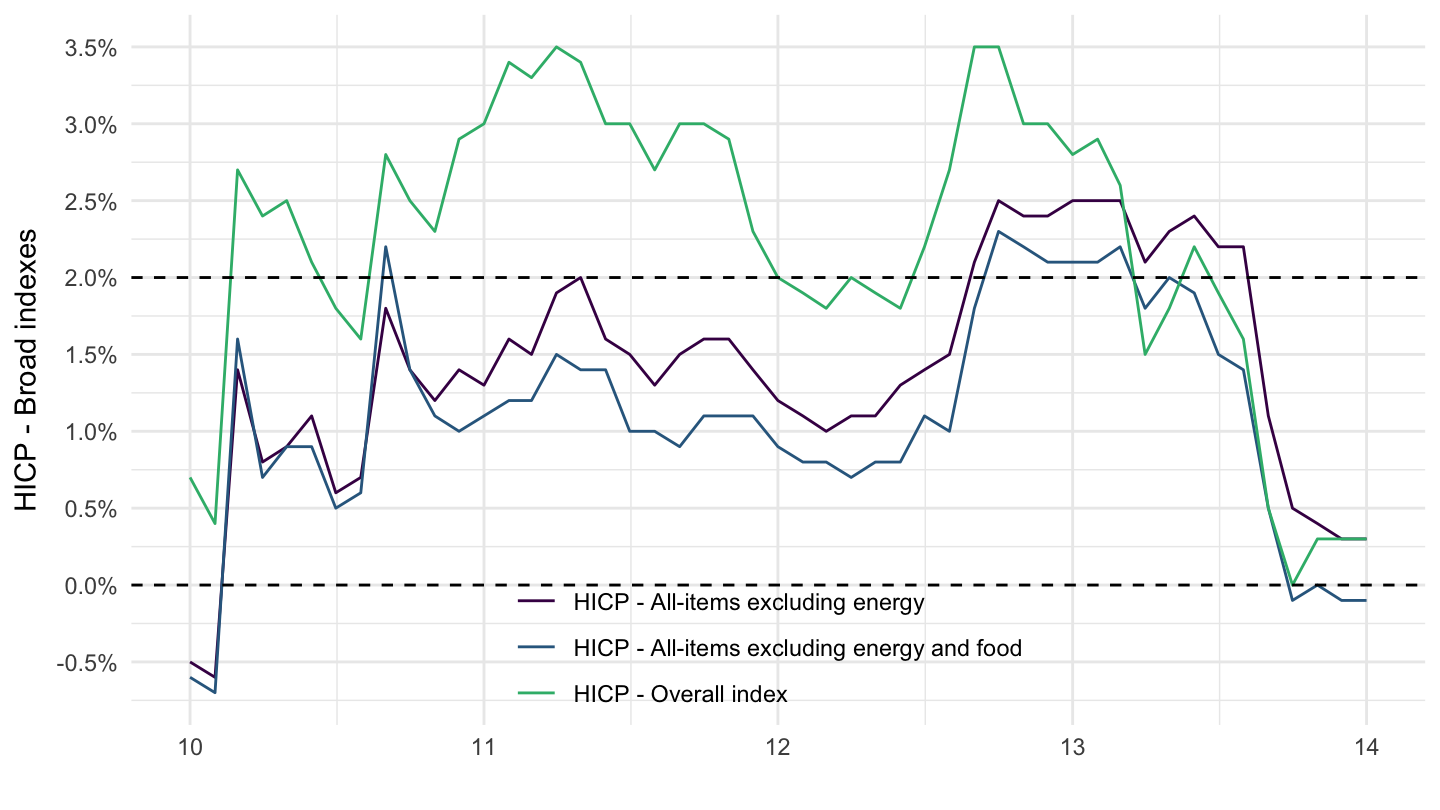
Greece
2010-2013
Code
ICP %>%
  filter(REF_AREA %in% c("GR"),
         # 000000: HICP - Overall index
         # XEF000: HICP - All-items excluding energy and food
         ICP_ITEM %in% c("000000", "XEF000", "XE0000"),
         # ANR: Annual Rate of Change
         ICP_SUFFIX == "ANR",
         FREQ == "M") %>%
  left_join(REF_AREA,  by = "REF_AREA") %>%
  month_to_date() %>%
  filter(!is.na(OBS_VALUE),
         date >= as.Date("2010-01-01"),
         date <= as.Date("2014-01-01")) %>%
  ggplot() + theme_minimal() + ylab("HICP - Broad indexes") + xlab("") +
  geom_line(aes(x = date, y = OBS_VALUE/100, color = TITLE)) +

  geom_hline(yintercept = 0.02, linetype = "dashed",  color = "black") +
  geom_hline(yintercept = 0, linetype = "dashed",  color = "black") +
  scale_x_date(breaks = seq(1920, 2100, 1) %>% paste0("-01-01") %>% as.Date,
               labels = date_format("%Y")) +
  theme(legend.position = c(0.2, 0.9),
        legend.title = element_blank()) +
  scale_y_continuous(breaks = 0.01*seq(-100, 200, 0.5),
                labels = percent_format(accuracy = 0.1))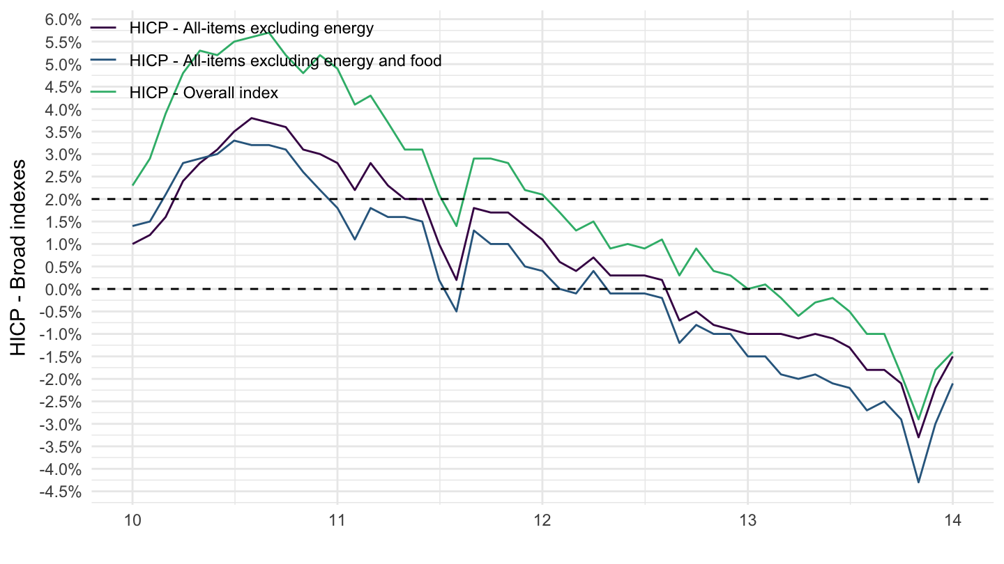
Germany Broad Indexes
1996-2021
Code
ICP %>%
  filter(REF_AREA %in% c("DE"),
         # 000000: HICP - Overall index
         # XEF000: HICP - All-items excluding energy and food
         ICP_ITEM %in% c("000000", "XEF000", "XE0000"),
         # ANR: Annual Rate of Change
         ICP_SUFFIX == "ANR",
         FREQ == "M") %>%
  left_join(REF_AREA,  by = "REF_AREA") %>%
  month_to_date() %>%
  filter(!is.na(OBS_VALUE),
         date >= as.Date("1996-01-01")) %>%
  ggplot() + theme_minimal() + ylab("HICP - Broad indexes") + xlab("") +
  geom_line(aes(x = date, y = OBS_VALUE/100, color = TITLE)) +

  geom_hline(yintercept = 0.02, linetype = "dashed",  color = "black") +
  geom_hline(yintercept = 0, linetype = "dashed",  color = "black") +
  scale_x_date(breaks = seq(1920, 2100, 2) %>% paste0("-01-01") %>% as.Date,
               labels = date_format("%Y")) +
  theme(legend.position = c(0.2, 0.9),
        legend.title = element_blank()) +
  scale_y_continuous(breaks = 0.01*seq(-100, 200, 0.5),
                labels = percent_format(accuracy = 0.1))
Annual - Euro area Broad Indexes
1996-2021
Code
ICP %>%
  filter(REF_AREA %in% c("U2"),
         # 000000: HICP - Overall index
         # XEF000: HICP - All-items excluding energy and food
         ICP_ITEM %in% c("XEFUN0", "XEF000", "XE0000"),
         # ANR: Annual Rate of Change
         ICP_SUFFIX == "INX",
         STS_INSTITUTION == 3,
         FREQ == "M") %>%
  left_join(REF_AREA,  by = "REF_AREA") %>%
  left_join(ICP_ITEM,  by = "ICP_ITEM") %>%
  month_to_date() %>%
  filter(!is.na(OBS_VALUE),
         date >= as.Date("1996-01-01"),
         month(date) == 1) %>%
  group_by(ICP_ITEM) %>%
  mutate(OBS_VALUE = 100*(OBS_VALUE/lag(OBS_VALUE, 1) - 1)) %>%
  select(KEY, ICP_ITEM, Icp_item, date, OBS_VALUE) %>%
  na.omit %>%
  ggplot() + theme_minimal() + ylab("HICP - Broad indexes") + xlab("") +
  geom_line(aes(x = date, y = OBS_VALUE/100, color = Icp_item)) +

  geom_hline(yintercept = 0.02, linetype = "dashed",  color = "black") +
  geom_hline(yintercept = 0, linetype = "dashed",  color = "black") +
  scale_x_date(breaks = seq(1920, 2100, 2) %>% paste0("-01-01") %>% as.Date,
               labels = date_format("%Y")) +
  theme(legend.position = c(0.75, 0.9),
        legend.title = element_blank()) +
  scale_y_continuous(breaks = 0.01*seq(0, 200, 0.5),
                labels = percent_format(accuracy = 0.1))
Monthly - Euro area Broad Indexes
1996-2021
Code
ICP %>%
  filter(REF_AREA %in% c("U2"),
         # 000000: HICP - Overall index
         # XEF000: HICP - All-items excluding energy and food
         ICP_ITEM %in% c("XEFUN0", "XEF000", "XE0000"),
         # ANR: Annual Rate of Change
         ICP_SUFFIX == "ANR",
         FREQ == "M") %>%
  left_join(REF_AREA,  by = "REF_AREA") %>%
  month_to_date() %>%
  filter(!is.na(OBS_VALUE),
         date >= as.Date("1996-01-01")) %>%
  ggplot() + theme_minimal() + ylab("HICP - Broad indexes") + xlab("") +
  geom_line(aes(x = date, y = OBS_VALUE/100, color = TITLE, linetype = TITLE)) +

  geom_hline(yintercept = 0.02, linetype = "dashed",  color = "black") +
  geom_hline(yintercept = 0, linetype = "dashed",  color = "black") +
  scale_x_date(breaks = seq(1920, 2100, 2) %>% paste0("-01-01") %>% as.Date,
               labels = date_format("%Y")) +
  theme(legend.position = c(0.75, 0.9),
        legend.title = element_blank()) +
  scale_y_continuous(breaks = 0.01*seq(0, 200, 0.5),
                labels = percent_format(accuracy = 0.1))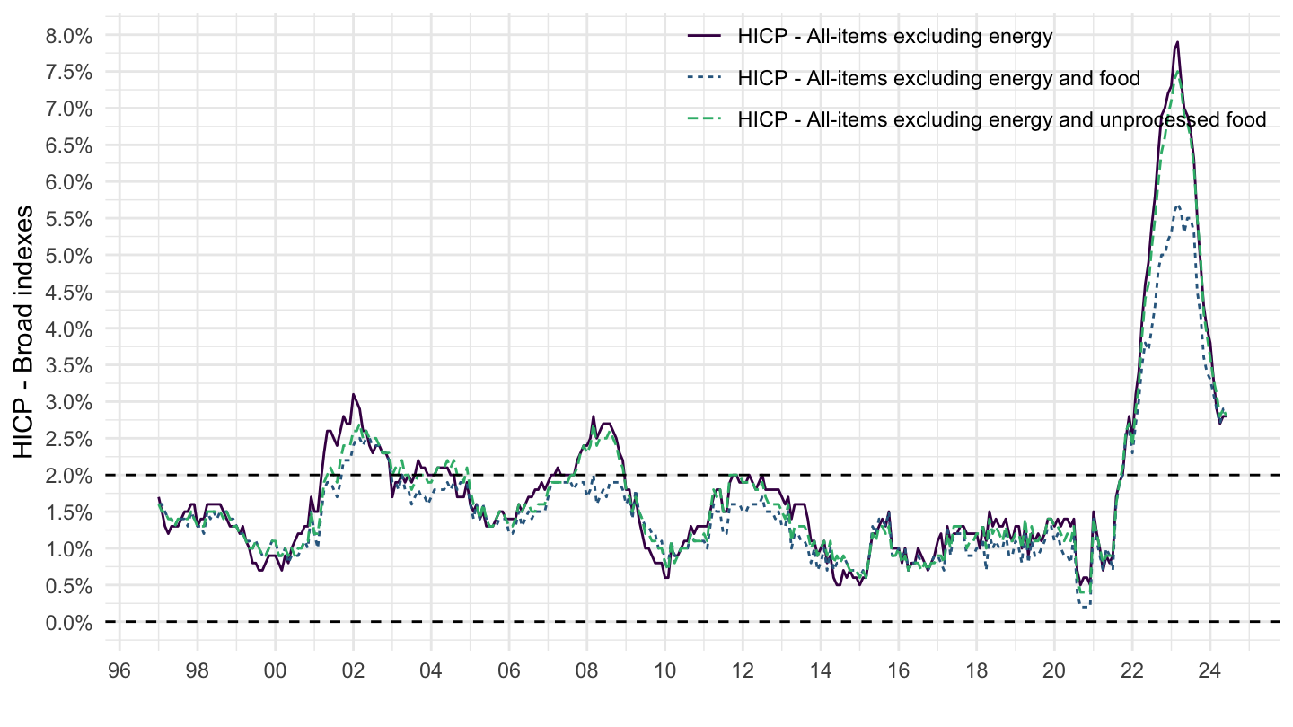
2009-2021
Code
ICP %>%
  filter(REF_AREA %in% c("U2"),
         # 000000: HICP - Overall index
         # XEF000: HICP - All-items excluding energy and food
         ICP_ITEM %in% c("XEFUN0", "XEF000", "XE0000"),
         # ANR: Annual Rate of Change
         ICP_SUFFIX == "ANR",
         FREQ == "M") %>%
  left_join(REF_AREA,  by = "REF_AREA") %>%
  month_to_date() %>%
  filter(!is.na(OBS_VALUE),
         date >= as.Date("2009-01-01")) %>%
  ggplot() + theme_minimal() + ylab("HICP - Broad indexes") + xlab("") +
  geom_line(aes(x = date, y = OBS_VALUE/100, color = TITLE, linetype = TITLE)) +

  geom_hline(yintercept = 0.02, linetype = "dashed",  color = "black") +
  geom_hline(yintercept = 0, linetype = "dashed",  color = "black") +
  scale_x_date(breaks = seq(1920, 2100, 1) %>% paste0("-01-01") %>% as.Date,
               labels = date_format("%Y")) +
  theme(legend.position = c(0.75, 0.9),
        legend.title = element_blank()) +
  scale_y_continuous(breaks = 0.01*seq(0, 200, 0.5),
                labels = percent_format(accuracy = 0.1))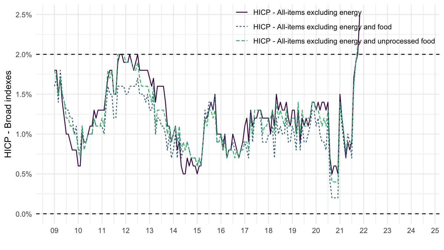
2009-2014
Code
ICP %>%
  filter(REF_AREA %in% c("U2"),
         # 000000: HICP - Overall index
         # XEF000: HICP - All-items excluding energy and food
         ICP_ITEM %in% c("XEFUN0", "000000", "XE0000"),
         # ANR: Annual Rate of Change
         ICP_SUFFIX == "ANR",
         FREQ == "M") %>%
  left_join(REF_AREA,  by = "REF_AREA") %>%
  month_to_date() %>%
  filter(!is.na(OBS_VALUE),
         date >= as.Date("2009-01-01"),
         date <= as.Date("2014-12-31")) %>%
  ggplot() + theme_minimal() + ylab("HICP - Broad indexes") + xlab("") +
  geom_line(aes(x = date, y = OBS_VALUE/100, color = TITLE, linetype = TITLE)) +

  geom_hline(yintercept = 0.02, linetype = "dashed",  color = "black") +
  scale_x_date(breaks = seq(1920, 2100, 1) %>% paste0("-01-01") %>% as.Date,
               labels = date_format("%Y")) +
  theme(legend.position = c(0.6, 0.2),
        legend.title = element_blank()) +
  scale_y_continuous(breaks = 0.01*seq(0, 200, 0.5),
                labels = percent_format(accuracy = 0.1)) +
  geom_vline(xintercept = as.Date("2011-04-07"), linetype = "dashed", color = "black") +
  geom_vline(xintercept = as.Date("2011-07-07"), linetype = "dashed", color = "black")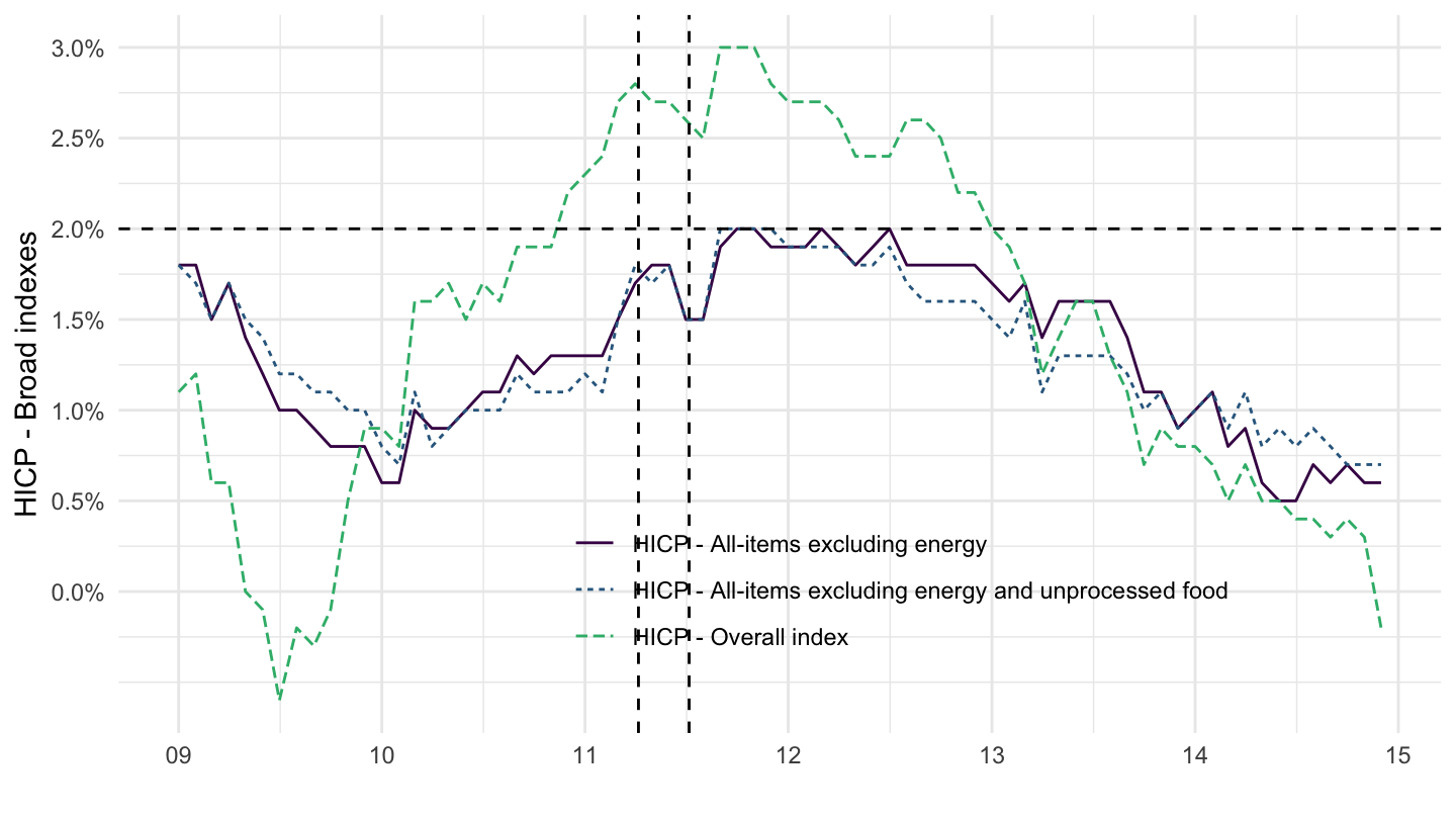
2013-2021
Code
ICP %>%
  filter(REF_AREA %in% c("U2"),
         # 000000: HICP - Overall index
         # XEF000: HICP - All-items excluding energy and food
         ICP_ITEM %in% c("XEFUN0", "000000", "XE0000"),
         # ANR: Annual Rate of Change
         ICP_SUFFIX == "ANR",
         FREQ == "M") %>%
  left_join(REF_AREA,  by = "REF_AREA") %>%
  month_to_date() %>%
  filter(!is.na(OBS_VALUE),
         date >= as.Date("2013-01-01"),
         date <= as.Date("2021-12-31")) %>%
  ggplot() + theme_minimal() + ylab("HICP - Broad indexes") + xlab("") +
  geom_line(aes(x = date, y = OBS_VALUE/100, color = TITLE)) +

  geom_hline(yintercept = 0.02, linetype = "dashed",  color = "black") +
  scale_x_date(breaks = seq(1920, 2100, 1) %>% paste0("-01-01") %>% as.Date,
               labels = date_format("%Y")) +
  theme(legend.position = c(0.3, 0.9),
        legend.title = element_blank()) +
  scale_y_continuous(breaks = 0.01*seq(0, 200, 0.5),
                labels = percent_format(accuracy = 0.1)) +
  geom_vline(xintercept = as.Date("2011-04-07"), linetype = "dashed", color = "black") +
  geom_vline(xintercept = as.Date("2011-07-07"), linetype = "dashed", color = "black")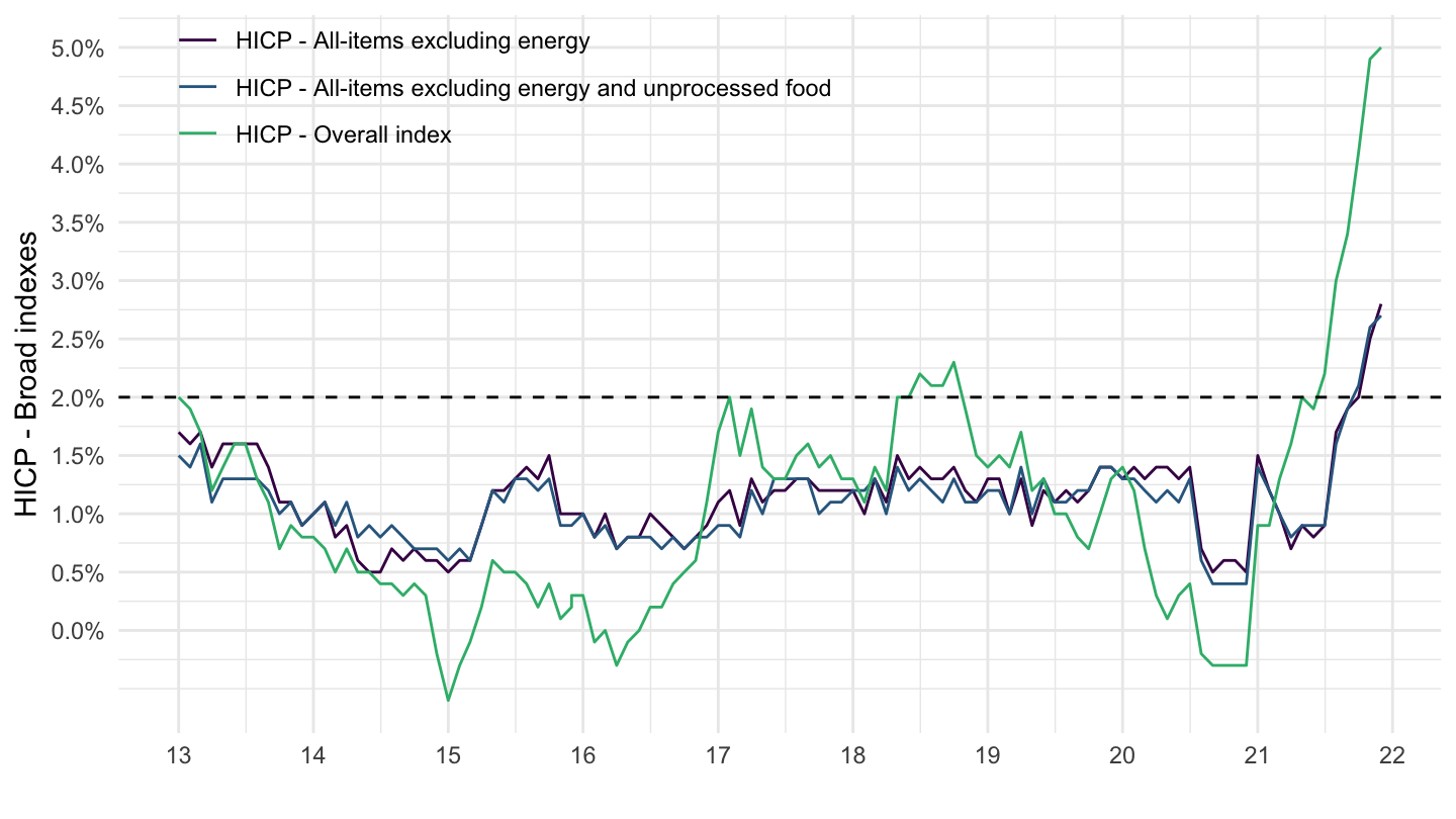
Euro area - Long
Code
ICP %>%
  filter(REF_AREA %in% c("U2"),
         # 000000: HICP - Overall index
         # XEF000: HICP - All-items excluding energy and food
         ICP_ITEM %in% c("000000"),
         # ANR: Annual Rate of Change
         ICP_SUFFIX == "ANR",
         FREQ == "M") %>%
  left_join(REF_AREA,  by = "REF_AREA") %>%
  month_to_date() %>%
  filter(!is.na(OBS_VALUE)) %>%
  ggplot() + theme_minimal() + ylab("HICP - Overall index") + xlab("") +
  geom_line(aes(x = date, y = OBS_VALUE/100, color = TITLE, linetype = TITLE)) +
  geom_hline(yintercept = 0.02, linetype = "dashed",  color = viridis(3)[2]) +
  scale_x_date(breaks = seq(1920, 2100, 5) %>% paste0("-01-01") %>% as.Date,
               labels = date_format("%Y")) +
  theme(legend.position = c(0.75, 0.8),
        legend.title = element_blank()) +
  scale_y_continuous(breaks = 0.01*seq(0, 200, 2),
                labels = percent_format(accuracy = 1))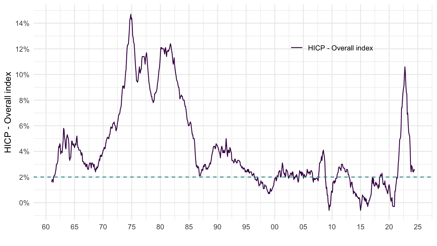
Germany, France, United Kinggom
Code
ICP %>%
  filter(REF_AREA %in% c("DE", "FR", "GB"),
         # 000000: HICP - Overall index
         ICP_ITEM == "000000",
         FREQ == "M",
         UNIT_INDEX_BASE == "2015 = 100") %>%
  left_join(REF_AREA,  by = "REF_AREA") %>%
  month_to_date() %>%
  filter(!is.na(OBS_VALUE)) %>%
  ggplot() +
  geom_line(aes(x = date, y = OBS_VALUE, color = Ref_area)) +

  theme_minimal() +
  scale_x_date(breaks = seq(1920, 2100, 2) %>% paste0("-01-01") %>% as.Date,
               labels = date_format("%Y")) +
  theme(legend.position = c(0.75, 0.3),
        legend.title = element_blank()) +
  scale_y_log10(breaks = seq(0, 200, 5),
                     labels = dollar_format(accuracy = 1, prefix = "")) +
  ylab("HICP - Overall index") + xlab("")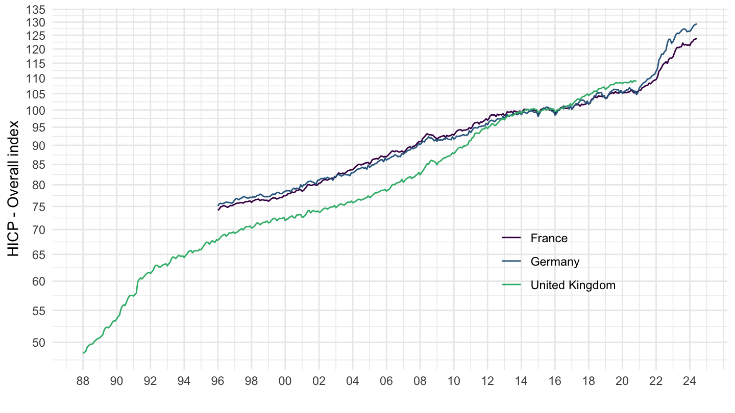
Decomposition between Services and Goods
France
Monthly
Code
ICP %>%
  filter(REF_AREA %in% c("FR"),
         # 000000: HICP - Overall index
         ICP_ITEM %in% c("SERV00", "041000", "IGXE00"),
         FREQ == "M",
         UNIT_INDEX_BASE == "2015 = 100",
         UNIT == "PURE_NUMB") %>%
  left_join(ICP_ITEM, by = "ICP_ITEM") %>%
  month_to_date() %>%
  filter(!is.na(OBS_VALUE)) %>%
  ggplot() +
  geom_line(aes(x = date, y = OBS_VALUE, color = Icp_item)) +

  theme_minimal() +
  scale_x_date(breaks = seq(1920, 2100, 2) %>% paste0("-01-01") %>% as.Date,
               labels = date_format("%Y")) +
  theme(legend.position = c(0.35, 0.85),
        legend.title = element_blank()) +
  scale_y_log10(breaks = seq(0, 200, 5),
                     labels = dollar_format(accuracy = 1, prefix = "")) +
  ylab("HICP - Overall index") + xlab("")
Annual
Code
ICP %>%
  filter(REF_AREA %in% c("FR"),
         # 000000: HICP - Overall index
         ICP_ITEM %in% c("SERV00", "041000", "IGXE00"),
         UNIT == "PURE_NUMB",
         FREQ == "A") %>%
  left_join(ICP_ITEM, by = "ICP_ITEM") %>%
  year_to_date() %>%
  group_by(ICP_ITEM) %>%
  mutate(OBS_VALUE = 100*OBS_VALUE/OBS_VALUE[date == as.Date("1996-01-01")]) %>%
  ggplot() + ylab("HICP - Overall index") + xlab("") + theme_minimal() +
  geom_line(aes(x = date, y = OBS_VALUE, color = Icp_item)) +

  scale_x_date(breaks = seq(1920, 2100, 2) %>% paste0("-01-01") %>% as.Date,
               labels = date_format("%Y")) +
  theme(legend.position = c(0.25, 0.15),
        legend.title = element_blank()) +
  scale_y_log10(breaks = seq(0, 200, 5),
                labels = dollar_format(accuracy = 1, prefix = ""))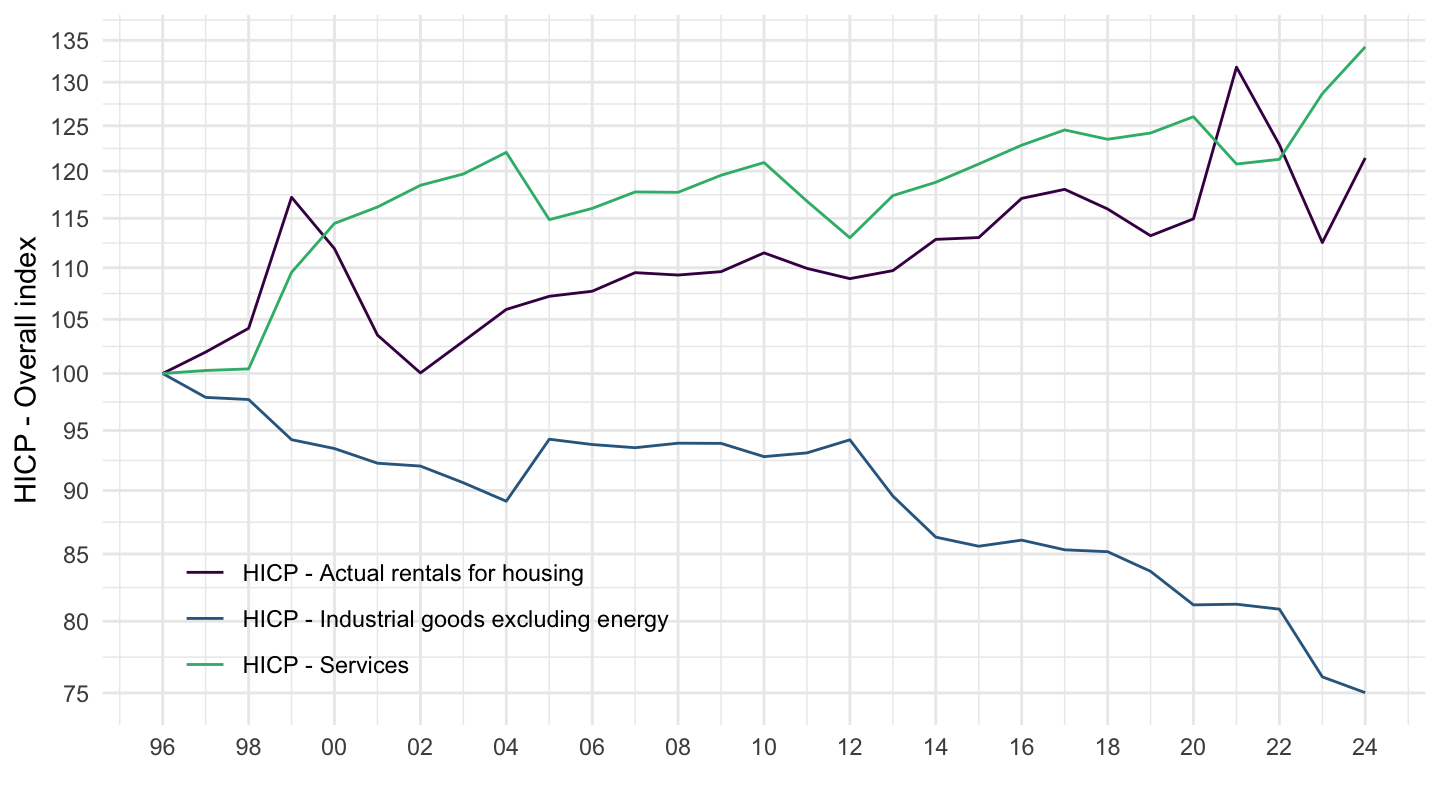
Germany
Code
ICP %>%
  filter(REF_AREA %in% c("DE"),
         # 000000: HICP - Overall index
         ICP_ITEM %in% c("SERV00", "041000", "IGXE00"),
         FREQ == "M",
         UNIT_INDEX_BASE == "2015 = 100",
         UNIT == "PURE_NUMB") %>%
  left_join(ICP_ITEM, by = "ICP_ITEM") %>%
  month_to_date() %>%
  filter(!is.na(OBS_VALUE)) %>%
  ggplot() +
  geom_line(aes(x = date, y = OBS_VALUE, color = Icp_item)) +

  theme_minimal() +
  scale_x_date(breaks = seq(1920, 2100, 2) %>% paste0("-01-01") %>% as.Date,
               labels = date_format("%Y")) +
  theme(legend.position = c(0.35, 0.85),
        legend.title = element_blank()) +
  scale_y_log10(breaks = seq(0, 200, 5),
                     labels = dollar_format(accuracy = 1, prefix = "")) +
  ylab("HICP - Overall index") + xlab("")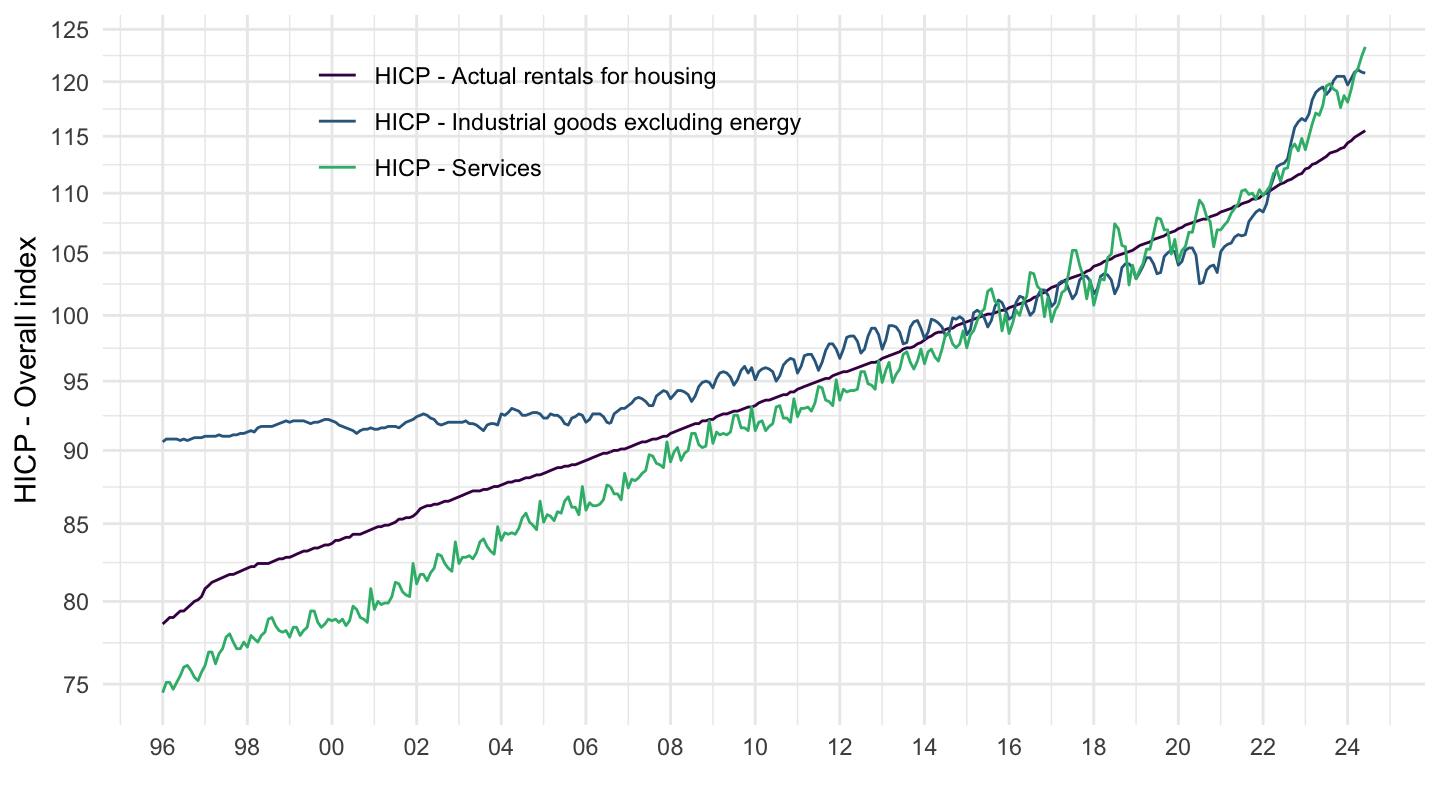
Greece
Code
ICP %>%
  filter(REF_AREA %in% c("GR"),
         # 000000: HICP - Overall index
         ICP_ITEM %in% c("SERV00", "041000", "IGXE00"),
         FREQ == "M",
         UNIT_INDEX_BASE == "2015 = 100",
         UNIT == "PURE_NUMB") %>%
  left_join(ICP_ITEM, by = "ICP_ITEM") %>%
  month_to_date() %>%
  filter(!is.na(OBS_VALUE)) %>%
  ggplot() +
  geom_line(aes(x = date, y = OBS_VALUE, color = Icp_item)) +

  theme_minimal() +
  scale_x_date(breaks = seq(1920, 2100, 2) %>% paste0("-01-01") %>% as.Date,
               labels = date_format("%Y")) +
  theme(legend.position = c(0.35, 0.85),
        legend.title = element_blank()) +
  scale_y_log10(breaks = seq(0, 200, 5),
                     labels = dollar_format(accuracy = 1, prefix = "")) +
  ylab("HICP - Overall index") + xlab("")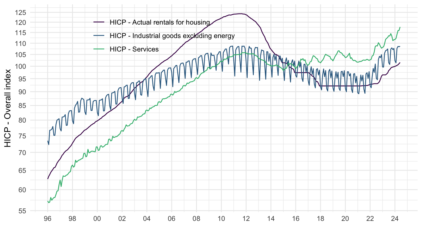
Portugal
Code
ICP %>%
  filter(REF_AREA %in% c("PT"),
         # 000000: HICP - Overall index
         ICP_ITEM %in% c("SERV00", "041000", "IGXE00"),
         FREQ == "M",
         UNIT_INDEX_BASE == "2015 = 100",
         UNIT == "PURE_NUMB") %>%
  left_join(ICP_ITEM, by = "ICP_ITEM") %>%
  month_to_date() %>%
  filter(!is.na(OBS_VALUE)) %>%
  ggplot() +
  geom_line(aes(x = date, y = OBS_VALUE, color = Icp_item)) +

  theme_minimal() +
  scale_x_date(breaks = seq(1920, 2100, 2) %>% paste0("-01-01") %>% as.Date,
               labels = date_format("%Y")) +
  theme(legend.position = c(0.35, 0.85),
        legend.title = element_blank()) +
  scale_y_log10(breaks = seq(0, 200, 5),
                     labels = dollar_format(accuracy = 1, prefix = "")) +
  ylab("HICP - Overall index") + xlab("")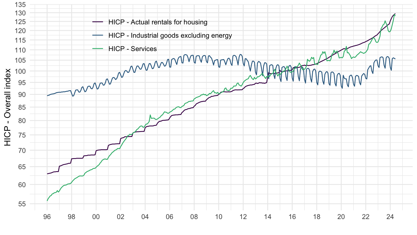
Further Decomposing
Germany
Code
ICP %>%
  filter(REF_AREA %in% c("DE"),
         # 000000: HICP - Overall index
         ICP_ITEM %in% c("110000", "120000", "030000", "041000"),
         FREQ == "M",
         UNIT_INDEX_BASE == "2015 = 100",
         UNIT == "PURE_NUMB") %>%
  left_join(ICP_ITEM, by = "ICP_ITEM") %>%
  month_to_date() %>%
  filter(!is.na(OBS_VALUE)) %>%
  ggplot() +
  geom_line(aes(x = date, y = OBS_VALUE, color = Icp_item)) +

  theme_minimal() +
  scale_x_date(breaks = seq(1920, 2100, 2) %>% paste0("-01-01") %>% as.Date,
               labels = date_format("%Y")) +
  theme(legend.position = c(0.35, 0.85),
        legend.title = element_blank()) +
  scale_y_log10(breaks = seq(0, 200, 5),
                     labels = dollar_format(accuracy = 1, prefix = "")) +
  ylab("HICP - Overall index") + xlab("")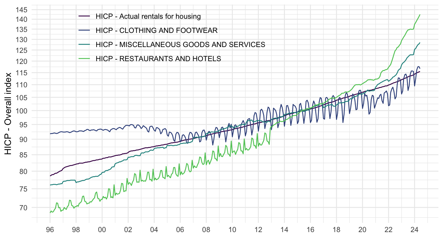
France
Code
ICP %>%
  filter(REF_AREA %in% c("FR"),
         # 000000: HICP - Overall index
         ICP_ITEM %in% c("110000", "120000", "030000", "041000"),
         FREQ == "M",
         UNIT_INDEX_BASE == "2015 = 100",
         UNIT == "PURE_NUMB") %>%
  left_join(ICP_ITEM, by = "ICP_ITEM") %>%
  month_to_date() %>%
  filter(!is.na(OBS_VALUE)) %>%
  ggplot() +
  geom_line(aes(x = date, y = OBS_VALUE, color = Icp_item)) +

  theme_minimal() +
  scale_x_date(breaks = seq(1920, 2100, 2) %>% paste0("-01-01") %>% as.Date,
               labels = date_format("%Y")) +
  theme(legend.position = c(0.75, 0.25),
        legend.title = element_blank()) +
  scale_y_log10(breaks = seq(0, 200, 5),
                     labels = dollar_format(accuracy = 1, prefix = "")) +
  ylab("HICP - Overall index") + xlab("")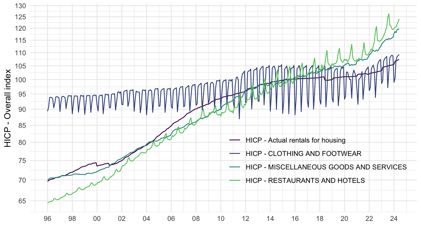
Greece
Code
ICP %>%
  filter(REF_AREA %in% c("GR"),
         # 000000: HICP - Overall index
         ICP_ITEM %in% c("110000", "120000", "030000", "041000"),
         FREQ == "M",
         UNIT_INDEX_BASE == "2015 = 100",
         UNIT == "PURE_NUMB") %>%
  left_join(ICP_ITEM, by = "ICP_ITEM") %>%
  month_to_date() %>%
  filter(!is.na(OBS_VALUE)) %>%
  ggplot() +
  geom_line(aes(x = date, y = OBS_VALUE, color = Icp_item)) +

  theme_minimal() +
  scale_x_date(breaks = seq(1920, 2100, 2) %>% paste0("-01-01") %>% as.Date,
               labels = date_format("%Y")) +
  theme(legend.position = c(0.75, 0.25),
        legend.title = element_blank()) +
  scale_y_log10(breaks = seq(0, 200, 5),
                     labels = dollar_format(accuracy = 1, prefix = "")) +
  ylab("HICP - Overall index") + xlab("")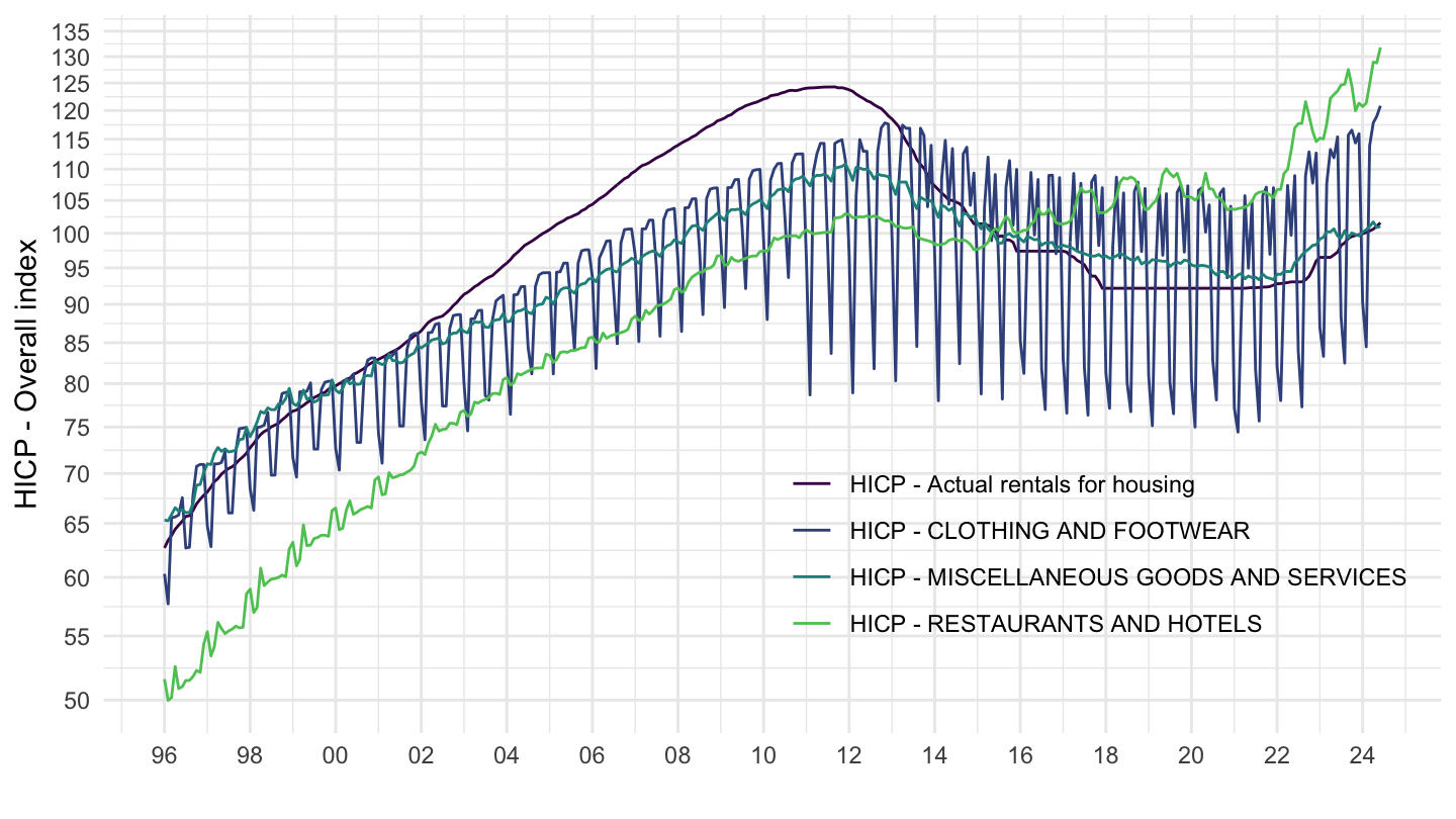
Portugal
Code
ICP %>%
  filter(REF_AREA %in% c("PT"),
         # 000000: HICP - Overall index
         ICP_ITEM %in% c("110000", "120000", "030000", "041000"),
         FREQ == "M",
         UNIT_INDEX_BASE == "2015 = 100",
         UNIT == "PURE_NUMB") %>%
  left_join(ICP_ITEM, by = "ICP_ITEM") %>%
  month_to_date() %>%
  filter(!is.na(OBS_VALUE)) %>%
  ggplot() +
  geom_line(aes(x = date, y = OBS_VALUE, color = Icp_item)) +

  theme_minimal() +
  scale_x_date(breaks = seq(1920, 2100, 2) %>% paste0("-01-01") %>% as.Date,
               labels = date_format("%Y")) +
  theme(legend.position = c(0.75, 0.25),
        legend.title = element_blank()) +
  scale_y_log10(breaks = seq(0, 200, 5),
                     labels = dollar_format(accuracy = 1, prefix = "")) +
  ylab("HICP - Overall index") + xlab("")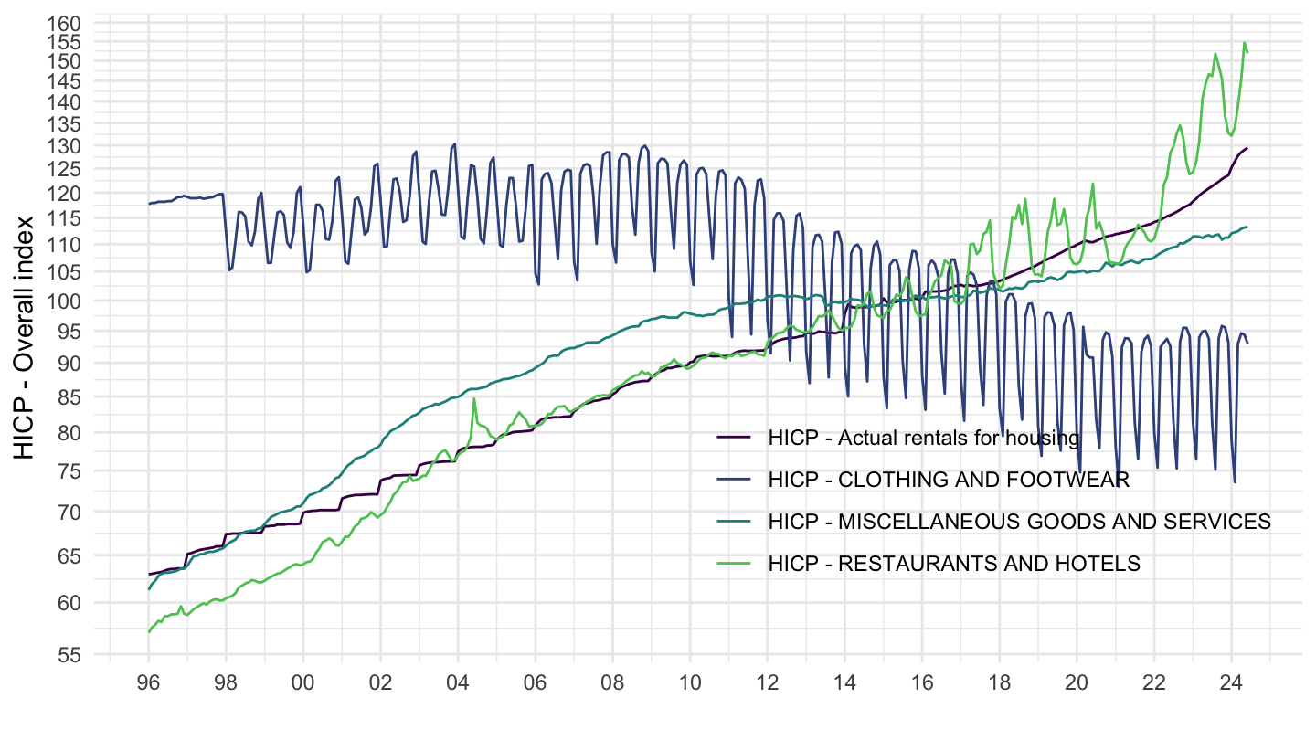
Price of Energy
Code
ICP %>%
  filter(REF_AREA %in% c("DE"),
         # 000000: HICP - Overall index
         ICP_ITEM %in% c("NRGY00", "ELGAS0", "045500"),
         FREQ == "M",
         ICP_SUFFIX == "INX") %>%
  left_join(ICP_ITEM, by = "ICP_ITEM") %>%
  month_to_date() %>%
  filter(!is.na(OBS_VALUE)) %>%
  ggplot() +
  geom_line(aes(x = date, y = OBS_VALUE, color = Icp_item)) +

  theme_minimal() +
  scale_x_date(breaks = seq(1920, 2100, 2) %>% paste0("-01-01") %>% as.Date,
               labels = date_format("%Y")) +
  theme(legend.position = c(0.75, 0.25),
        legend.title = element_blank()) +
  scale_y_log10(breaks = seq(0, 200, 5),
                     labels = dollar_format(accuracy = 1, prefix = "")) +
  ylab("HICP - Overall index") + xlab("")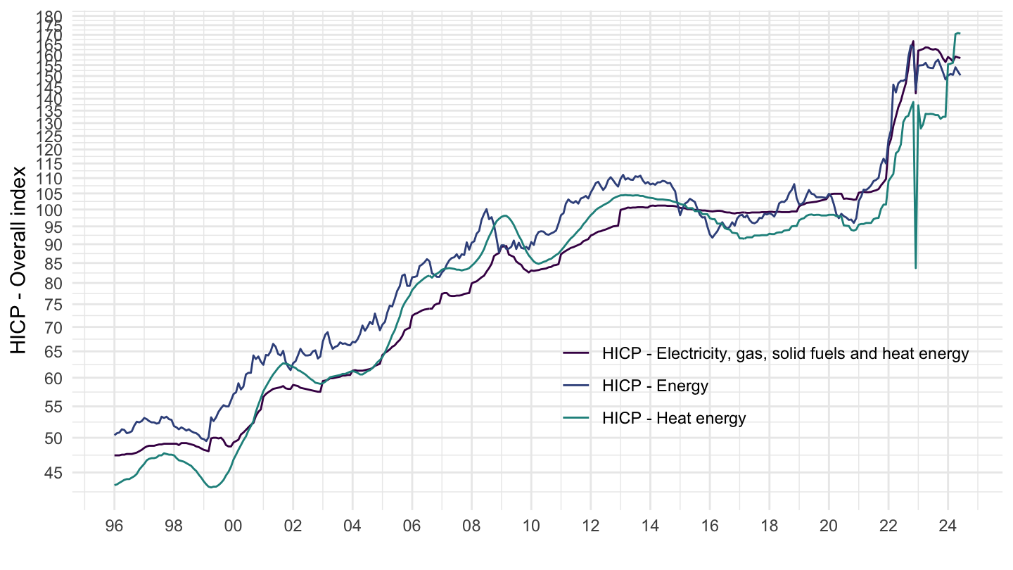
Deflation in Greece
Code
ICP %>%
  filter(REF_AREA %in% c("GR"),
         FREQ == "M",
         UNIT_INDEX_BASE == "2015 = 100",
         UNIT == "PURE_NUMB") %>%
  left_join(ICP_ITEM, by = "ICP_ITEM") %>%
  month_to_date() %>%
  filter(!is.na(OBS_VALUE),
         date %in% as.Date(paste0(c(2012, 2014), "-01-01"))) %>%
  select(date, ICP_ITEM, TITLE, OBS_VALUE) %>%
  group_by(ICP_ITEM, TITLE) %>%
  summarise(`% change` = round(100*(OBS_VALUE[2] - OBS_VALUE[1])/OBS_VALUE[1], 1)) %>%
  arrange(`% change`) %>%
  {if (is_html_output()) datatable(., filter = 'top', rownames = F) else .}