Trafic aérien commercial mensuel par liaison (série LSN) - trafic-aerien-liaisons

Name: Trafic aérien commercial mensuel par liaison (série LSN)
Creator: François Geerolf

Auteur

Source : DGAC, data.gouv.fr. Trafic par segment (LSN_SEG : NAT intérieur, INTL international), faisceau (LSN_FSC) et pays (LSN_2). Passagers locaux : LSN_PAX.

Segments et faisceaux

Passagers locaux, intérieur vs. international

Code

`trafic-aerien-liaisons` |>
  mutate(annee = year(date)) |>
  group_by(annee, LSN_SEG) |>
  summarise(pax = sum(LSN_PAX, na.rm = TRUE) / 1e6, .groups = "drop") |>
  mutate(date = as.Date(paste0(annee, "-01-01")),
         Segment = ifelse(LSN_SEG == "NAT", "Intérieur", "International")) |>
  ggplot(aes(x = date, y = pax, fill = Segment)) +
  geom_area() + theme_minimal() + xlab("") + ylab("Millions de passagers") +
  scale_fill_manual(values = c("#2166ac", "#e08214")) +
  scale_x_date(date_breaks = "5 years", labels = date_format("%Y")) +
  theme(legend.position = "bottom", legend.title = element_blank())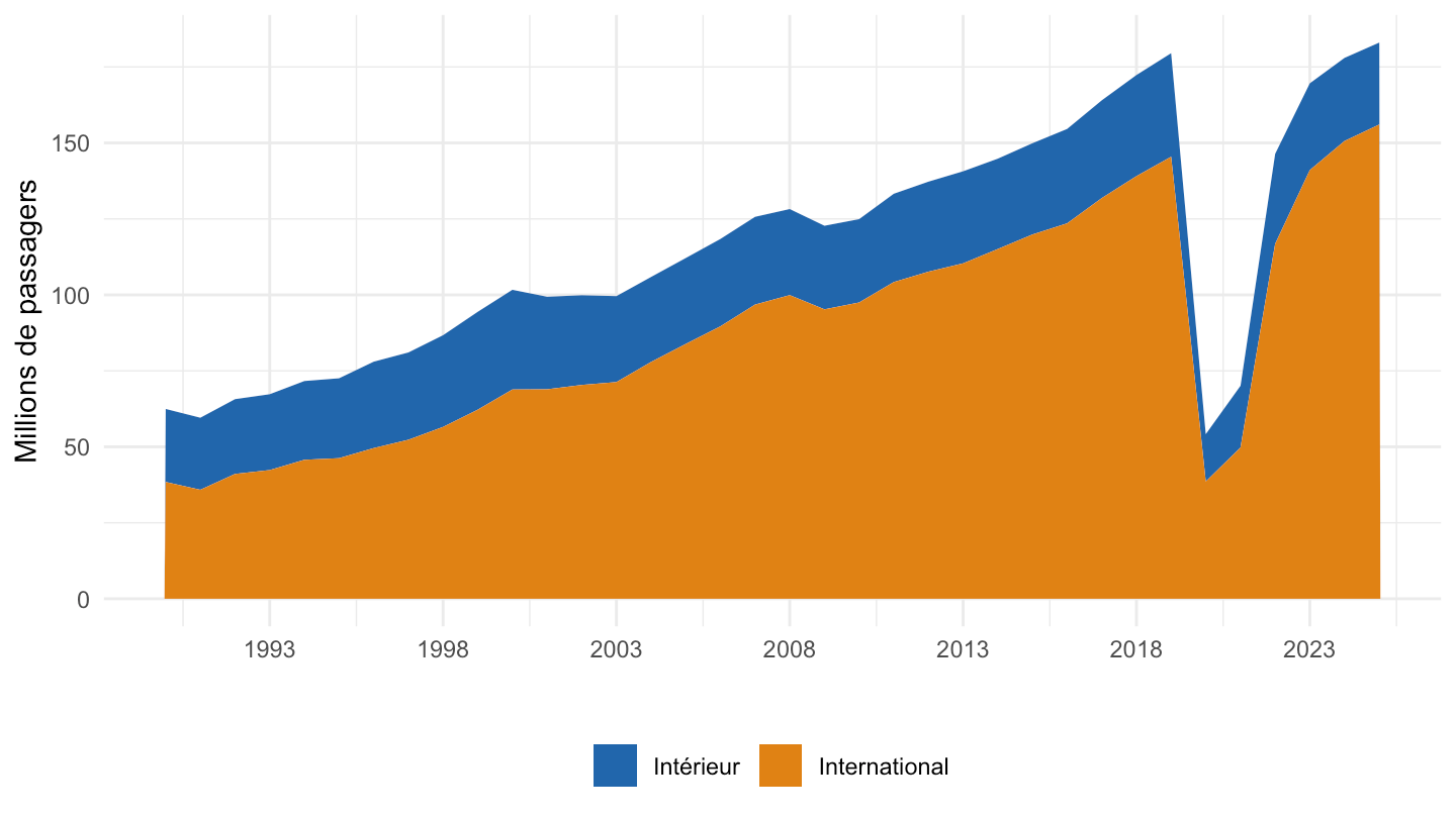

Par faisceau

Code

faisceaux_lab <- c(MET_RAD = "Métropole, radiales", MET_TRA = "Métropole, transversales",
                   MET_OM = "Métropole - Outre-mer", OM_OM = "Intérieur Outre-mer",
                   MET_INTL = "International, Métropole", OM_INTL = "International, Outre-mer")
`trafic-aerien-liaisons` |>
  mutate(annee = year(date)) |>
  group_by(annee, LSN_FSC) |>
  summarise(pax = sum(LSN_PAX, na.rm = TRUE) / 1e6, .groups = "drop") |>
  mutate(date = as.Date(paste0(annee, "-01-01")), Faisceau = faisceaux_lab[LSN_FSC]) |>
  ggplot(aes(x = date, y = pax, color = Faisceau)) +
  geom_line() + theme_minimal() + xlab("") + ylab("Millions de passagers") +
  scale_x_date(date_breaks = "5 years", labels = date_format("%Y")) +
  theme(legend.position = "bottom", legend.title = element_blank())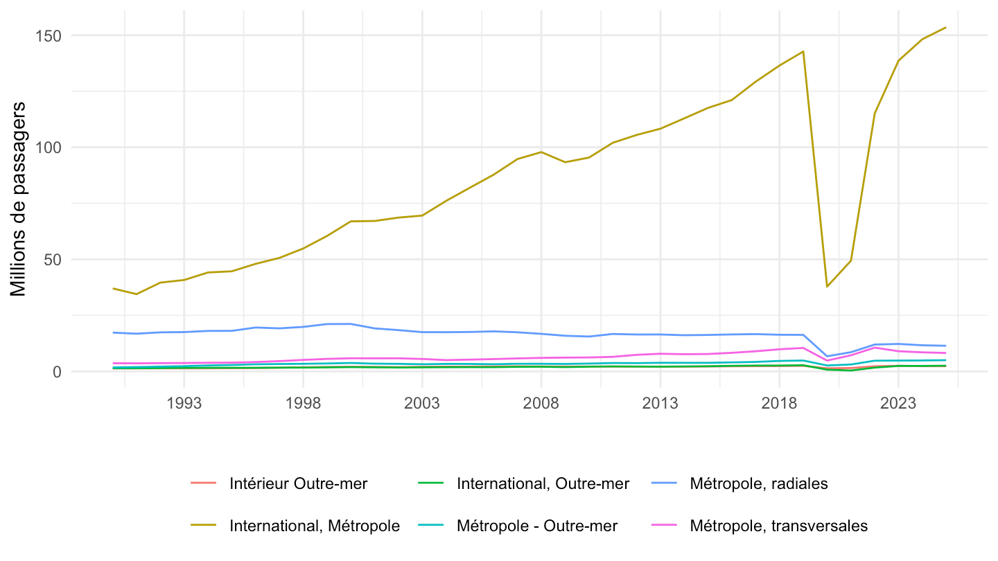

Radiales et transversales (indice 100 = 2000)

Code

`trafic-aerien-liaisons` |>
  filter(LSN_FSC %in% c("MET_RAD", "MET_TRA")) |>
  mutate(annee = year(date)) |>
  group_by(annee, LSN_FSC) |>
  summarise(pax = sum(LSN_PAX, na.rm = TRUE), .groups = "drop") |>
  group_by(LSN_FSC) |>
  mutate(indice = 100 * pax / pax[annee == 2000], Faisceau = faisceaux_lab[LSN_FSC],
         date = as.Date(paste0(annee, "-01-01"))) |>
  ggplot(aes(x = date, y = indice, color = Faisceau)) +
  geom_line() + theme_minimal() + xlab("") + ylab("Passagers (2000 = 100)") +
  scale_x_date(date_breaks = "5 years", labels = date_format("%Y")) +
  theme(legend.position = "bottom", legend.title = element_blank())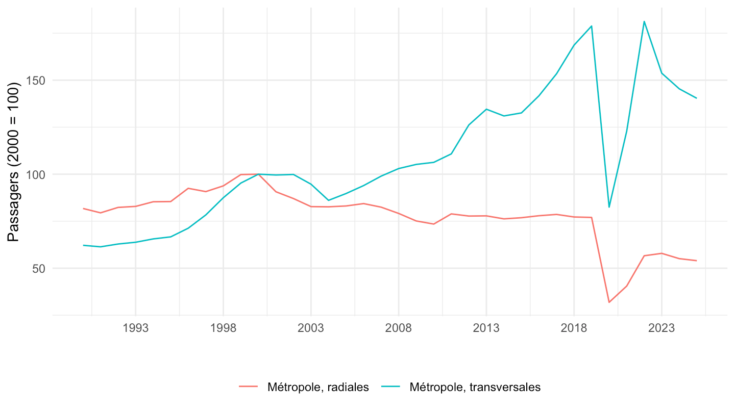

International

Par continent de destination

Code

`trafic-aerien-liaisons` |>
  filter(LSN_SEG == "INTL") |>
  mutate(annee = year(date)) |>
  group_by(annee, LSN_2_CONT) |>
  summarise(pax = sum(LSN_PAX, na.rm = TRUE) / 1e6, .groups = "drop") |>
  mutate(date = as.Date(paste0(annee, "-01-01")), Continent = str_to_title(LSN_2_CONT)) |>
  ggplot(aes(x = date, y = pax, fill = Continent)) +
  geom_area() + theme_minimal() + xlab("") + ylab("Millions de passagers") +
  scale_fill_viridis_d(end = 0.9) +
  scale_x_date(date_breaks = "5 years", labels = date_format("%Y")) +
  theme(legend.position = "bottom", legend.title = element_blank())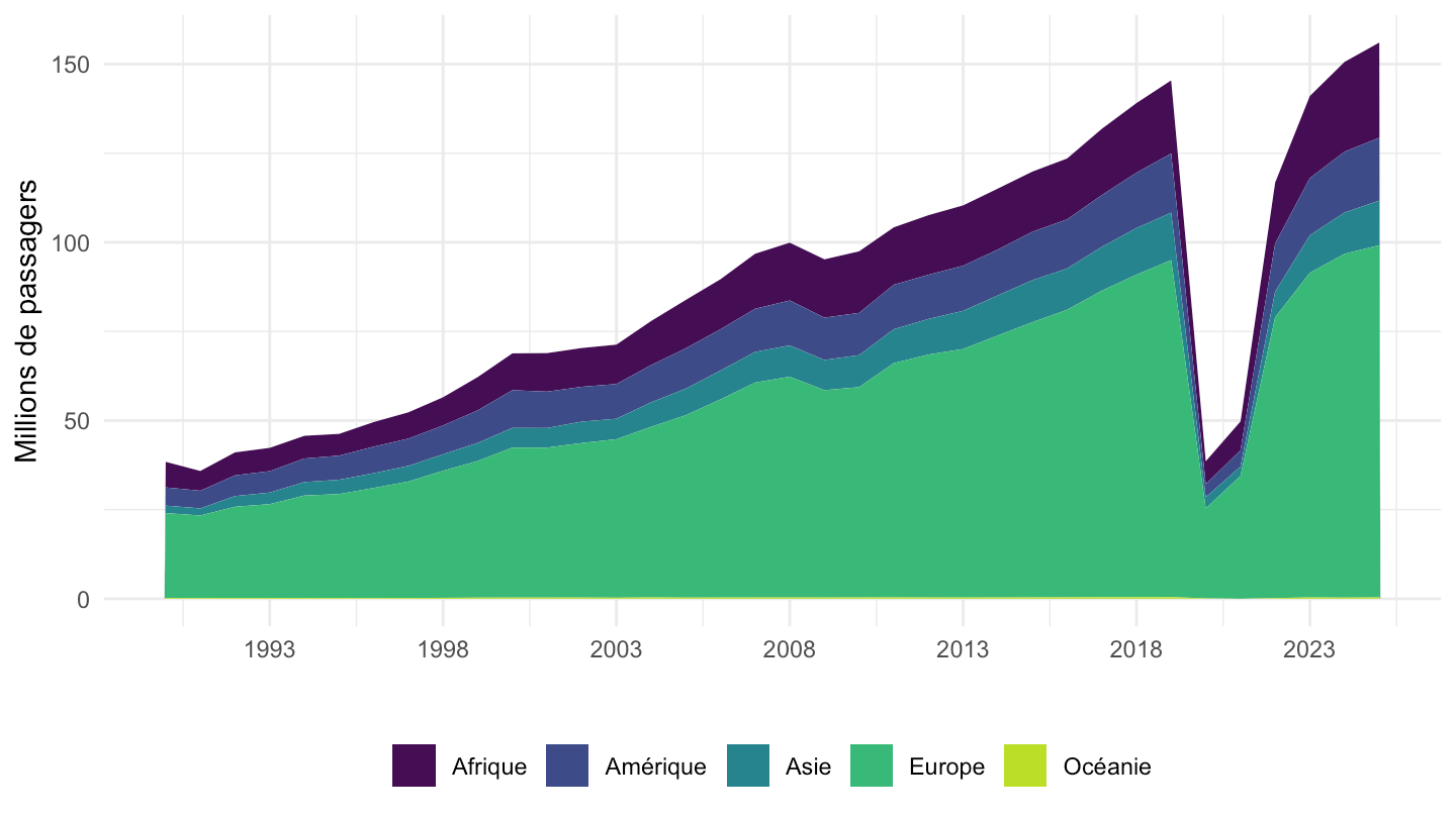

Principaux pays de destination, 2025 et 2019 (départs de Métropole)

Code

pays <- `trafic-aerien-liaisons` |>
  filter(LSN_FSC == "MET_INTL", year(date) %in% c(2019, 2025), !grepl("_AUTRE", LSN_2)) |>
  group_by(LSN_2, annee = year(date)) |>
  summarise(pax = sum(LSN_PAX, na.rm = TRUE) / 1e6, .groups = "drop")
top <- pays |> filter(annee == 2025) |> slice_max(pax, n = 15) |> pull(LSN_2)
pays |>
  filter(LSN_2 %in% top) |>
  mutate(LSN_2 = fct_reorder(str_to_title(LSN_2), pax, .fun = max)) |>
  ggplot(aes(x = LSN_2, y = pax, fill = factor(annee))) +
  geom_col(position = "dodge") + coord_flip() + theme_minimal() +
  xlab("") + ylab("Millions de passagers") +
  scale_fill_manual(values = c("#9ecae1", "#08519c")) +
  theme(legend.position = "bottom", legend.title = element_blank())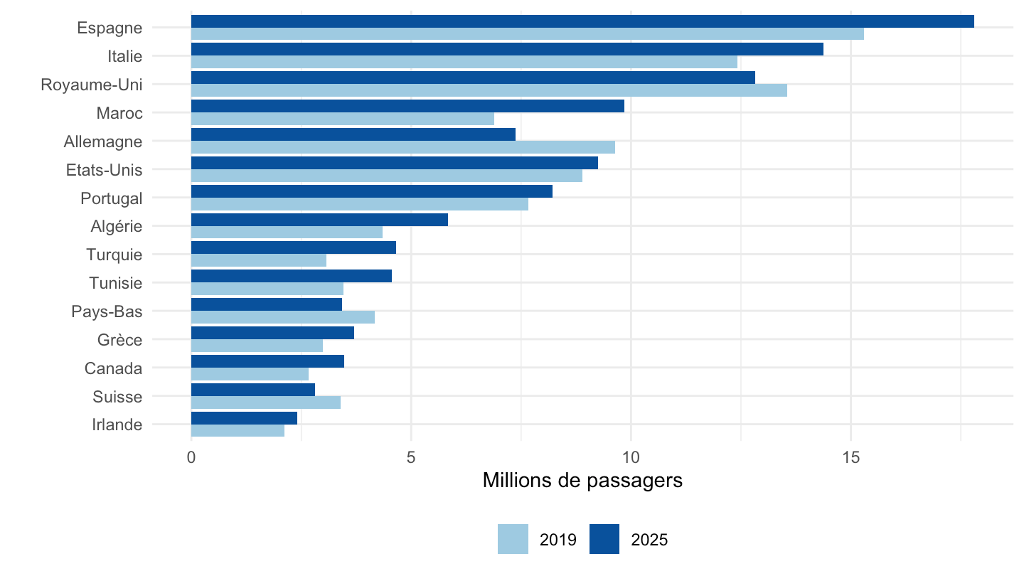

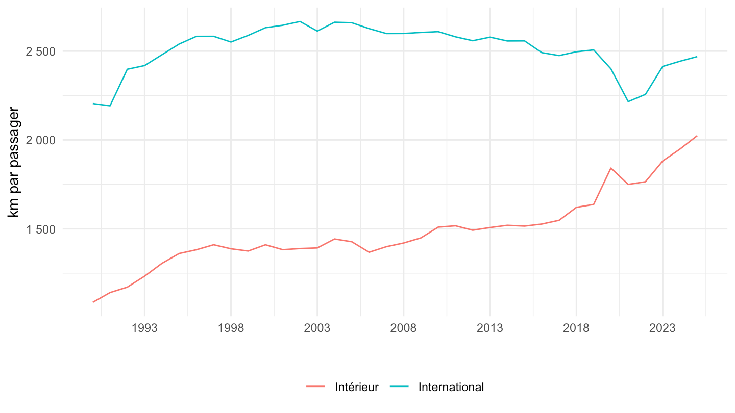
Distance moyenne par passager (km)

Code

`trafic-aerien-liaisons` |>
  mutate(annee = year(date)) |>
  group_by(annee, LSN_SEG) |>
  summarise(km = sum(LSN_PKT, na.rm = TRUE) / sum(LSN_PAX, na.rm = TRUE), .groups = "drop") |>
  mutate(date = as.Date(paste0(annee, "-01-01")),
         Segment = ifelse(LSN_SEG == "NAT", "Intérieur", "International")) |>
  ggplot(aes(x = date, y = km, color = Segment)) +
  geom_line() + theme_minimal() + xlab("") + ylab("km par passager") +
  scale_x_date(date_breaks = "5 years", labels = date_format("%Y")) +
  scale_y_continuous(labels = fr) +
  theme(legend.position = "bottom", legend.title = element_blank())