Indices des prix du transport aérien de passagers (IPTAP) - indices-des-prix-du-transport-aerien

Name: Indices des prix du transport aérien de passagers (IPTAP)
Creator: François Geerolf

Auteur

Source : DGAC, data.gouv.fr ; méthodologie : ministère. Indices mensuels (billets aller-retour au départ de France, structure de consommation constante). Trois séries : courant (depuis 2017, base 2023 = 100), 2012-2025 (base 2023 = 100) et 2012-2024 (base 2017 = 100).

Code

# série la plus longue en base 2023 : 2012-2025 complétée par la série courante
longue <- bind_rows(
  `indices-des-prix-du-transport-aerien` |> filter(serie == "courant"),
  `indices-des-prix-du-transport-aerien` |> filter(serie == "2012-2025") |>
    anti_join(`indices-des-prix-du-transport-aerien` |> filter(serie == "courant"), by = c("date", "faisceau")))

Ensemble des départs de France

Indice des prix (base 100 = 2023), 2012-

Code

longue |>
  filter(faisceau == "FRA_ENS") |>
  ggplot(aes(x = date, y = value)) +
  geom_line() + theme_minimal() + xlab("") + ylab("Indice des prix (2023 = 100)") +
  scale_x_date(date_breaks = "2 years", labels = date_format("%Y"))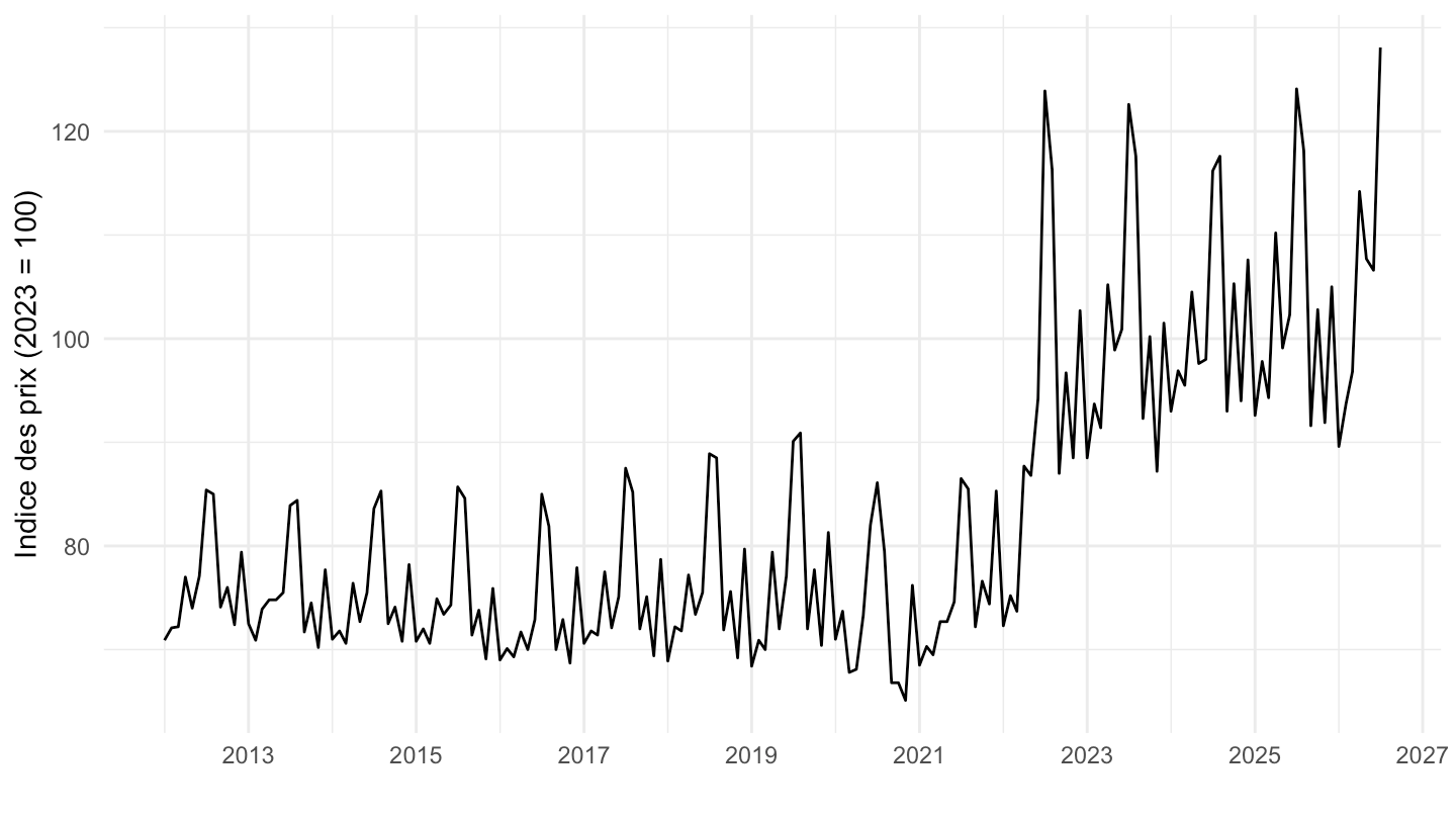

Glissement annuel

Code

longue |>
  filter(faisceau %in% c("FRA_ENS", "MET_INTER_TOT", "MET_INTAL_TOT")) |>
  arrange(faisceau_label, date) |>
  group_by(faisceau_label) |>
  mutate(glissement = value / lag(value, 12) - 1) |>
  filter(!is.na(glissement)) |>
  ggplot(aes(x = date, y = glissement, color = faisceau_label)) +
  geom_hline(yintercept = 0, linewidth = 0.3) +
  geom_line() + theme_minimal() + xlab("") + ylab("Glissement annuel") +
  scale_x_date(date_breaks = "2 years", labels = date_format("%Y")) +
  scale_y_continuous(labels = percent_format(accuracy = 1)) +
  theme(legend.position = "bottom", legend.title = element_blank()) +
  guides(color = guide_legend(ncol = 1))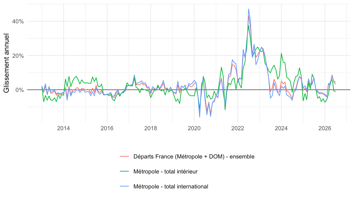

Par faisceau

Départs de Métropole : intérieur, moyen-courrier, long-courrier

Code

longue |>
  filter(faisceau %in% c("MET_INTER_TOT", "MET_INTAL_MC", "MET_INTAL_LC")) |>
  ggplot(aes(x = date, y = value, color = faisceau_label)) +
  geom_line() + theme_minimal() + xlab("") + ylab("Indice des prix (2023 = 100)") +
  scale_x_date(date_breaks = "2 years", labels = date_format("%Y")) +
  theme(legend.position = "bottom", legend.title = element_blank()) +
  guides(color = guide_legend(ncol = 1))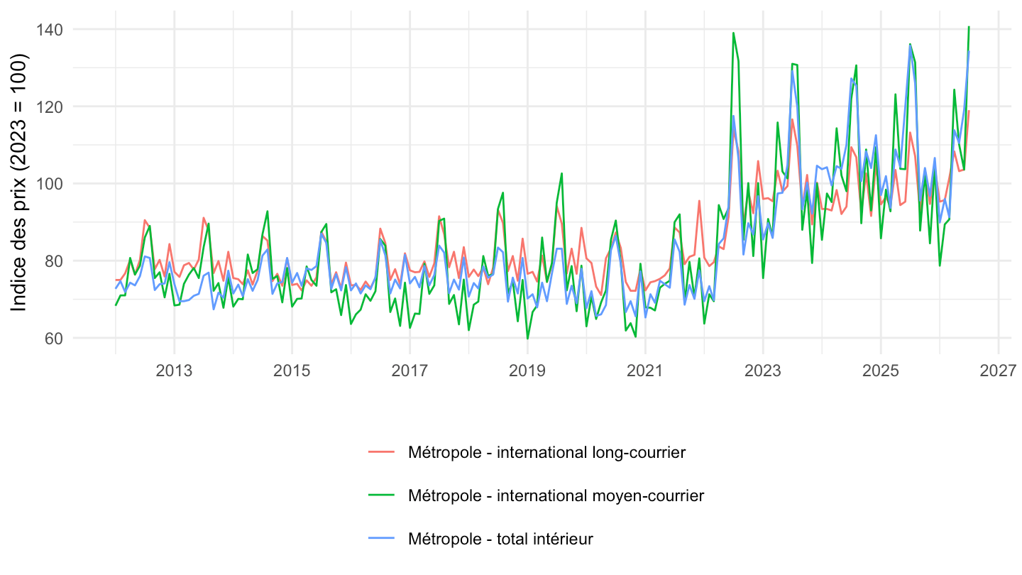

Métropole - Outre-mer vs. intérieur Métropole

Code

longue |>
  filter(faisceau %in% c("MET_INTER_MET", "MET_INTER_OM", "DOM_ENS")) |>
  ggplot(aes(x = date, y = value, color = faisceau_label)) +
  geom_line() + theme_minimal() + xlab("") + ylab("Indice des prix (2023 = 100)") +
  scale_x_date(date_breaks = "2 years", labels = date_format("%Y")) +
  theme(legend.position = "bottom", legend.title = element_blank()) +
  guides(color = guide_legend(ncol = 1))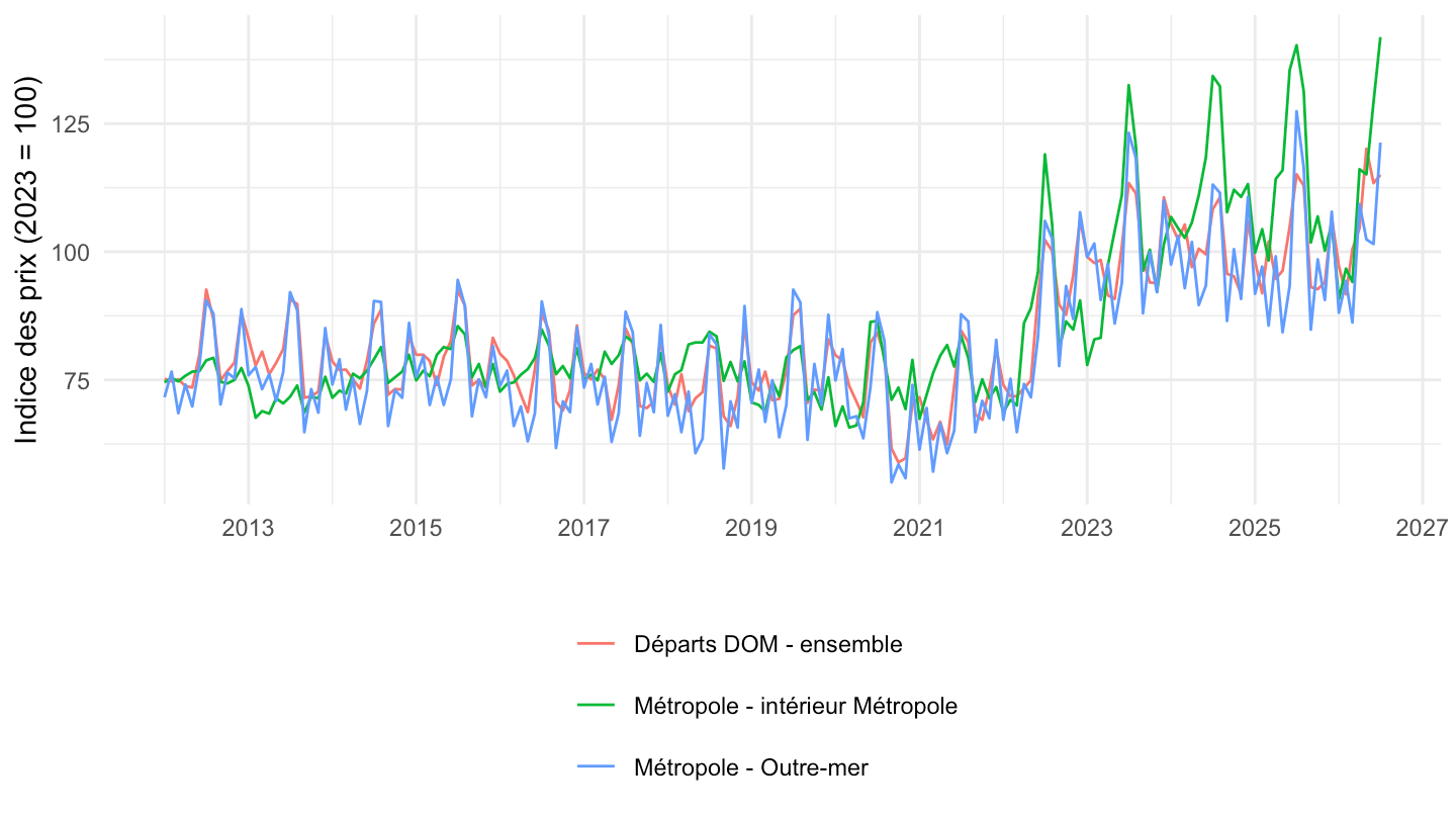

Saisonnalité

Profil mensuel de l’indice d’ensemble (indice rapporté à la moyenne annuelle)

Code

longue |>
  filter(faisceau == "FRA_ENS", year(date) %in% c(2017:2019, 2023:2025)) |>
  mutate(annee = year(date), mois = month(date),
         periode = ifelse(annee <= 2019, "2017-2019", "2023-2025")) |>
  group_by(annee) |>
  mutate(relatif = value / mean(value)) |>
  group_by(periode, mois) |>
  summarise(relatif = mean(relatif), .groups = "drop") |>
  ggplot(aes(x = mois, y = relatif, color = periode)) +
  geom_line() + geom_point(size = 0.8) + theme_minimal() +
  xlab("") + ylab("Indice / moyenne de l'année") +
  scale_x_continuous(breaks = 1:12, labels = month.abb) +
  theme(legend.position = "bottom", legend.title = element_blank())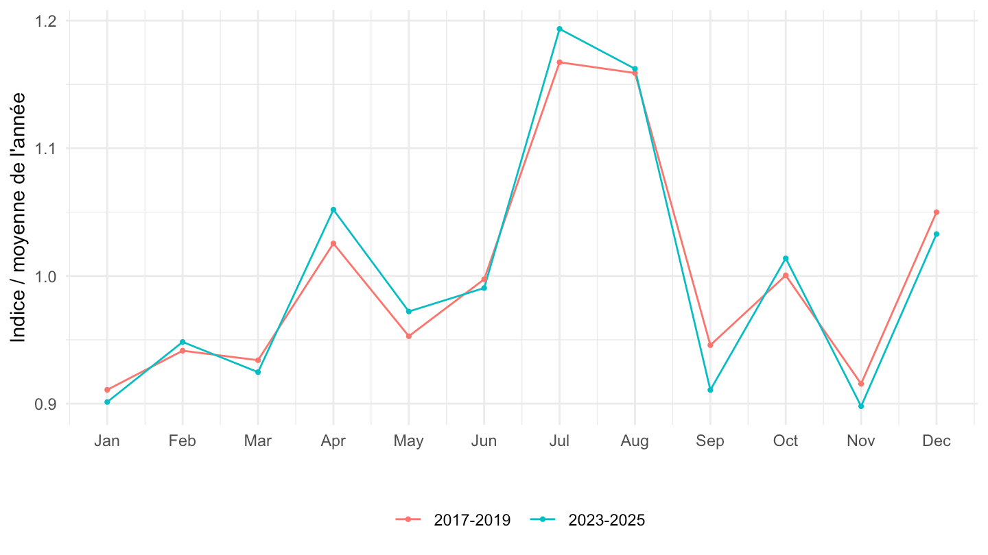

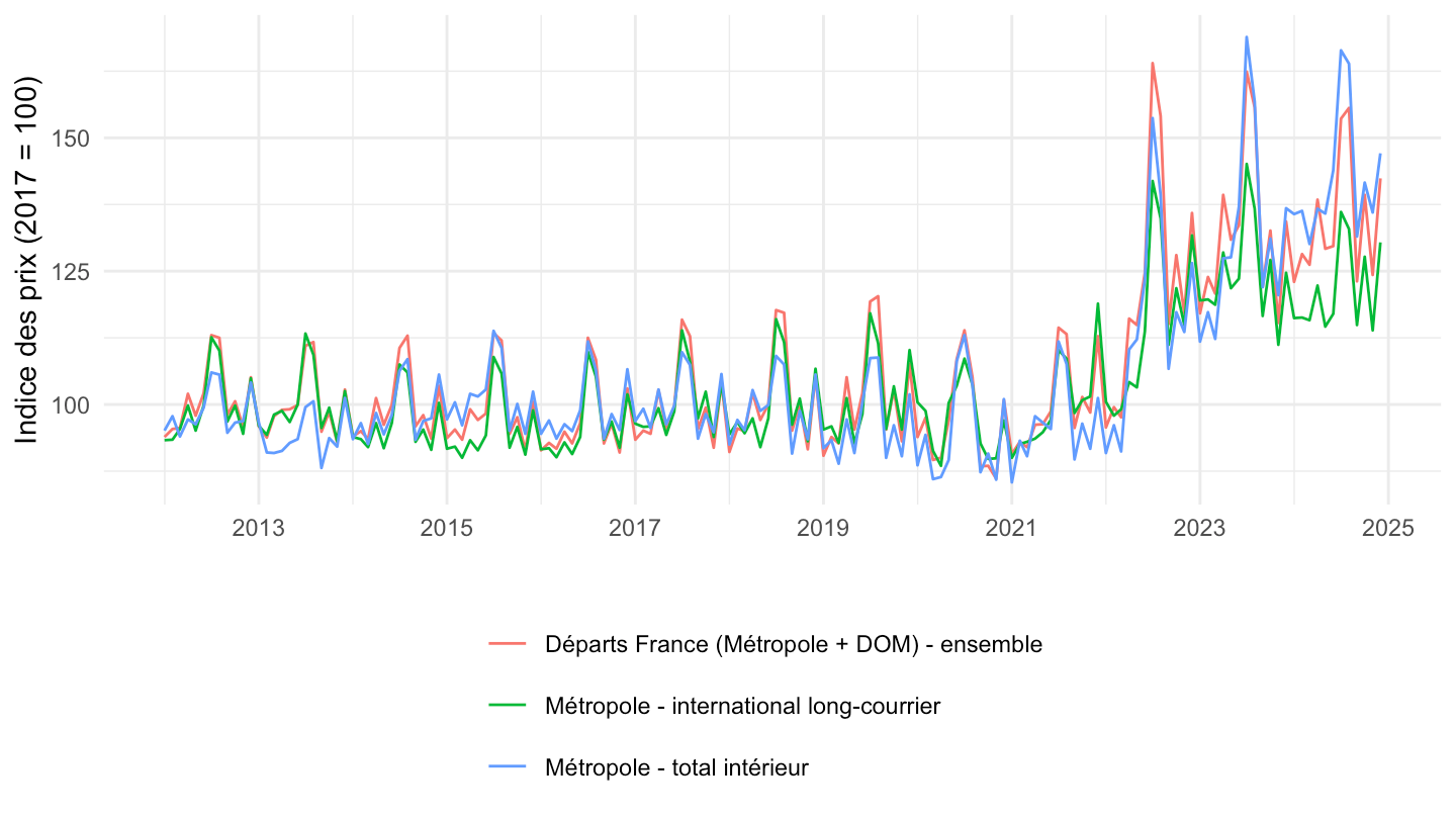
Série en base 2017

Code

`indices-des-prix-du-transport-aerien` |>
  filter(serie == "2012-2024", faisceau %in% c("FRA_ENS", "MET_INTAL_LC", "MET_INTER_TOT")) |>
  ggplot(aes(x = date, y = value, color = faisceau_label)) +
  geom_line() + theme_minimal() + xlab("") + ylab("Indice des prix (2017 = 100)") +
  scale_x_date(date_breaks = "2 years", labels = date_format("%Y")) +
  theme(legend.position = "bottom", legend.title = element_blank()) +
  guides(color = guide_legend(ncol = 1))