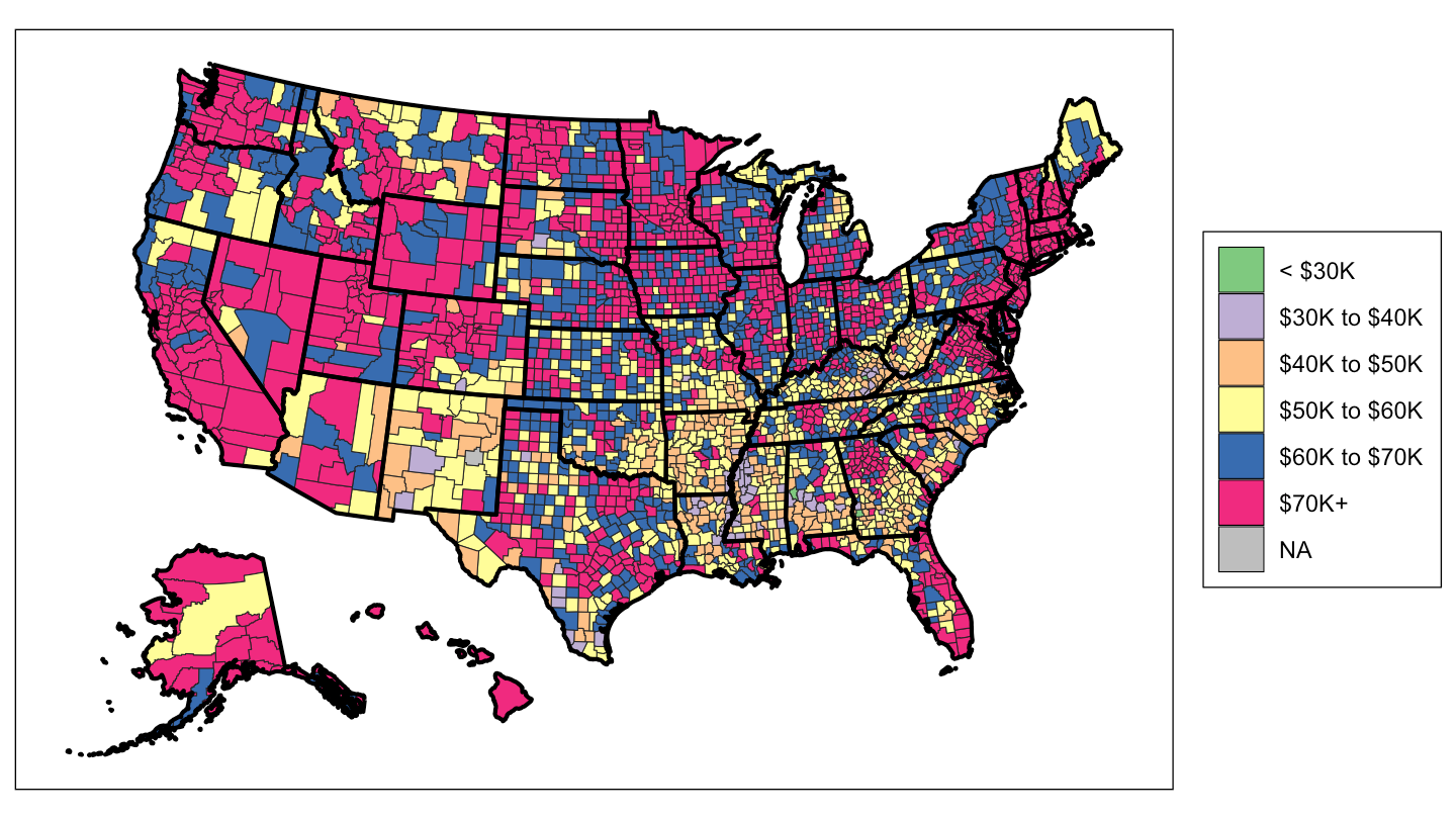
(ref:county-median-income) Median Income by County (Source: 2013-2017 ACS)
Code
get_acs(geography ="county", variables ="B19013_001") |>mutate(region = GEOID |>as.numeric()) |>select(region, value = estimate) |>mutate(value =case_when(value <30000~"< $30K", value >=30000& value <40000~"$30K to $40K", value >=40000& value <50000~"$40K to $50K", value >=50000& value <60000~"$50K to $60K", value >=60000& value <70000~"$60K to $70K", value >=70000~"$70K+")) |>county_choropleth()
(ref:county-median-income)
2000 Median Rents
To plot our first map, we use 2000 census county-level data on median rents. First, load tidycensus as well as choroplethr. Second, get a key for the Census API here, input it to census_key, and run the following in a R chunk:
Code
census_api_key(census_key)
Finally, plot median rents by county in the 2000 Census:
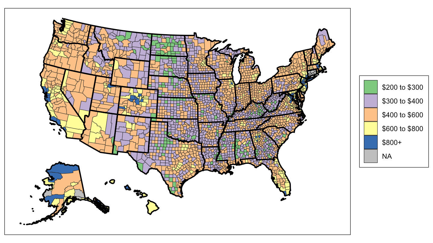
(ref:county-rents-census-2000) Census-Level Median Rent (Source: 2000 Census)
Code
get_decennial(geography ="county", variables ="H063001", year =2000) |>mutate(region = GEOID |>as.numeric()) |>mutate(value =case_when(value <200~"$0 to $200", value >=200& value <300~"$200 to $300", value >=300& value <400~"$300 to $400", value >=400& value <600~"$400 to $600", value >=600& value <800~"$600 to $800", value >=800~"$800+")) |>county_choropleth()