Last observation: 2024 (N = 96030)
First observation: 1984 (N = 10358)
Last data update: 15 oct. 2026, 22:19
Last compile: 15 oct. 2026, 22:25
First choose demographics:
Demographics: LB01 - By Quantile, LB02 - By Income
Characteristics: for each demographic type (e.g. 01), list of groups. (All, 1st quantile etc.)
Then choose item:
Category: EXPEND - Expenditures, or INCOME - Income and Taxes
Subcategory:
Item:
cx.demographics %>%
{if (is_html_output()) print_table(.) else .}| demographics_code | demographics_text | display_level | selectable | sort_sequence |
|---|---|---|---|---|
| LB01 | Quintiles of income before taxes | 0 | T | 100 |
| LB02 | Income before taxes | 0 | T | 200 |
| LB04 | Age of reference person | 0 | T | 300 |
| LB05 | Size of consumer unit | 0 | T | 400 |
| LB06 | Composition of consumer unit | 0 | T | 400 |
| LB07 | Number of earners | 0 | T | 500 |
| LB09 | Race of reference person | 0 | T | 700 |
| LB10 | Hispanic or Latino origin of reference person | 0 | T | 800 |
| LB11 | Region of residence | 0 | T | 900 |
| LB12 | Occupation of reference person | 0 | T | 1000 |
| LB13 | Education of reference person | 0 | T | 1100 |
| LB14 | Highest education level of any member | 0 | T | 1200 |
| LB15 | Deciles of income before taxes | 0 | T | 1300 |
| LB16 | Generation of reference person | 0 | T | 1600 |
| LB17 | Housing tenure | 0 | T | 1700 |
| LB18 | Type of area | 0 | T | 1800 |
| LB19 | Type of area | 0 | T | 1900 |
| LB20 | Population size of area of residence | 0 | T | 2000 |
| LB21 | Selected age of reference person | 0 | T | 2100 |
cx.characteristics %>%
{if (is_html_output()) datatable(., filter = 'top', rownames = F) else .}cx.category %>%
{if (is_html_output()) print_table(.) else .}| category_code | category_text | display_level | selectable | sort_sequence |
|---|---|---|---|---|
| ADDENDA | Assets and liabilities, and other financial info | 0 | T | 300 |
| CUCHARS | Consumer Characteristics | 0 | T | 400 |
| EXPEND | Expenditures | 0 | T | 100 |
| INCOME | Income and Taxes | 0 | T | 200 |
cx.subcategory %>%
  {if (is_html_output()) datatable(., filter = 'top', rownames = F) else .}
cx.item %>%
{if (is_html_output()) datatable(., filter = 'top', rownames = F) else .}cx.series |>
filter(demographics_code == "LB01",
item_code %in% c("INCAFTTX", "HOUSING", "INSPENSN", "TOTALEXP", "OWNMORTG")) |>
inner_join(cx.data.1.AllData |>
filter(year == 2016), by = "series_id") |>
inner_join(cx.characteristics |>
select(1, 2, 3), by = c("characteristics_code", "demographics_code")) |>
select(characteristics_code, characteristics_text, item_code, value) |>
spread(item_code, value) %>%
{if (is_html_output()) print_table(.) else .}| characteristics_code | characteristics_text | HOUSING | INCAFTTX | INSPENSN | OWNMORTG | TOTALEXP |
|---|---|---|---|---|---|---|
| 01 | All Consumer Units | 18886 | 64175 | 6831 | 2889 | 57311 |
| 02 | Lowest 20 percent income quintile | 10267 | 11832 | 645 | 545 | 25138 |
| 03 | Second 20 percent income quintile | 13552 | 29423 | 1766 | 977 | 36770 |
| 04 | Third 20 percent income quintile | 16315 | 47681 | 4227 | 1910 | 47664 |
| 05 | Fourth 20 percent income quintile | 20687 | 75065 | 8262 | 3707 | 64910 |
| 06 | Highest 20 percent income quintile | 33653 | 157215 | 19302 | 7325 | 112221 |
cx.series |>
  filter(demographics_code == "LB15",
         item_code %in% c("INCAFTTX", "HOUSING", "INSPENSN", "TOTALEXP", "OWNMORTG")) |>
  inner_join(cx.data.1.AllData |>
              filter(year == 2016), by = "series_id") |>
  inner_join(cx.characteristics |>
              select(1, 2, 3), by = c("characteristics_code", "demographics_code")) |>
  select(characteristics_code, characteristics_text, item_code, value) |>
  spread(item_code, value) %>%
{if (is_html_output()) print_table(.) else .}| characteristics_code | characteristics_text | HOUSING | INCAFTTX | INSPENSN | OWNMORTG | TOTALEXP |
|---|---|---|---|---|---|---|
| 01 | All consumer units | 18886 | 64175 | 6831 | 2889 | 57311 |
| 02 | Lowest 10 percent | 9567 | 6774 | 644 | 512 | 23588 |
| 03 | Second 10 percent | 10961 | 16841 | 645 | 579 | 26675 |
| 04 | Third 10 percent | 12829 | 25423 | 1411 | 760 | 34221 |
| 05 | Fourth 10 percent | 14271 | 33404 | 2120 | 1193 | 39308 |
| 06 | Fifth 10 percent | 15511 | 42410 | 3290 | 1547 | 43975 |
| 07 | Sixth 10 percent | 17119 | 52949 | 5164 | 2272 | 51351 |
| 08 | Seventh 10 percent | 19285 | 66676 | 7058 | 3198 | 59395 |
| 09 | Eighth 10 percent | 22085 | 83424 | 9461 | 4215 | 70411 |
| 10 | Ninth 10 percent | 26719 | 108743 | 13278 | 5564 | 87432 |
| 11 | Highest 10 percent | 40547 | 205391 | 25290 | 9075 | 136873 |
cx.series |>
  filter(demographics_code == "LB02",
         item_code %in% c("INCAFTTX", "HOUSING", "INSPENSN", "TOTALEXP", "OWNMORTG")) |>
  inner_join(cx.data.1.AllData |>
              filter(year == 2016), by = "series_id") |>
  inner_join(cx.characteristics |>
              select(1, 2, 3), by = c("characteristics_code", "demographics_code")) |>
  select(characteristics_code, characteristics_text, item_code, value) |>
  spread(item_code, value) |>
  filter(!is.na(INCAFTTX)) %>%
{if (is_html_output()) print_table(.) else .}| characteristics_code | characteristics_text | HOUSING | INCAFTTX | INSPENSN | OWNMORTG | TOTALEXP |
|---|---|---|---|---|---|---|
| 01 | All Consumer Units | 18886 | 64175 | 6831 | 2889 | 57311 |
| 07 | $30,000 to $39,999 before tax income | 14533 | 34381 | 2222 | 1274 | 40144 |
| 08 | $40,000 to $49,999 before tax income | 15575 | 43047 | 3400 | 1554 | 44150 |
| 09 | $50,000 to $69,999 before tax income | 17331 | 54782 | 5307 | 2451 | 52088 |
| 18 | Less than $15,000 | 9698 | 8732 | 614 | 551 | 23657 |
| 19 | $15,000 to $29,999 | 12268 | 23012 | 1161 | 678 | 31913 |
| 20 | $70,000 to $99,999 | 20564 | 74744 | 8270 | 3632 | 65086 |
| 21 | $100,000 to $149,999 | 26003 | 103504 | 12543 | 5299 | 84154 |
| 22 | $150,000 to $199,999 | 33319 | 140130 | 17609 | 7391 | 109516 |
| 23 | $200,000 and more | 46076 | 254890 | 31079 | 10333 | 158896 |
cx.series |>
  filter(demographics_code == "LB15",
         characteristics_code == "01") |>
  inner_join(cx.data.1.AllData |>
              filter(year == 2016), by = "series_id") |>
  inner_join(cx.item |>
              select(2, 3), by = c("item_code")) |>
  select(3, 4, 5, item_text, value) |>
  arrange(-value) %>%
{if (is_html_output()) datatable(., filter = 'top', rownames = F) else .}cx.series |>
filter(demographics_code == "LB15",
item_code %in% c("INCAFTTX", "HOUSING", "PENSIONS", "TOTALEXP", "OWNMORTG")) |>
inner_join(cx.data.1.AllData |>
filter(year == 2016), by = "series_id") |>
inner_join(cx.characteristics |>
select(1, 2, 3), by = c("characteristics_code", "demographics_code")) |>
select(characteristics_text, item_code, value) |>
spread(item_code, value) |>
transmute(characteristics_text,
INCAFTTX,
`Saving` = INCAFTTX - TOTALEXP,
`Total Saving (incl. Pensions)` = INCAFTTX - TOTALEXP + PENSIONS) |>
gather(variable, value, -1, -2) |>
ggplot() + geom_line(aes(x = INCAFTTX/1000, y = value/1000, color = variable)) +
theme_minimal() + xlab("Income after taxes") + ylab("Saving") +
theme(legend.position = c(0.45, 0.9),
legend.title = element_blank()) +
scale_x_continuous(breaks = seq(0, 200, 20),
labels = dollar_format(suffix = "K", accuracy = 1)) +
scale_color_manual(values = viridis(3)[1:2]) +
scale_y_continuous(breaks = seq(-100, 200, 10),
labels = dollar_format(suffix = "K", accuracy = 1))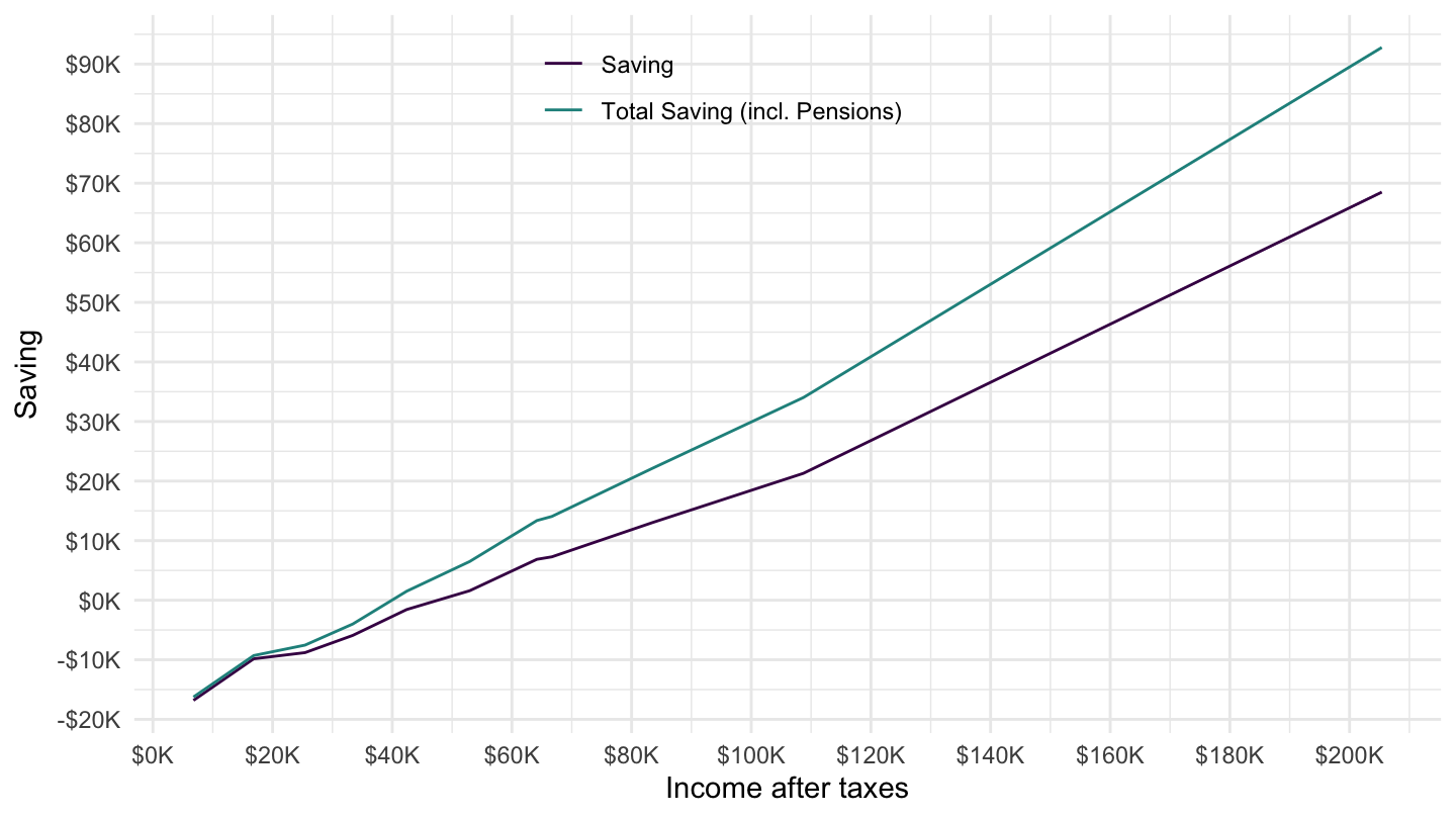
cx.series |>
  filter(demographics_code == "LB15",
         item_code %in% c("INCAFTTX", "HOUSING", "PENSIONS", "TOTALEXP", "OWNMORTG")) |>
  inner_join(cx.data.1.AllData |>
              filter(year == 2016), by = "series_id") |>
  inner_join(cx.characteristics |>
              select(1, 2, 3), by = c("characteristics_code", "demographics_code")) |>
  select(characteristics_text, item_code, value) |>
  spread(item_code, value) |>
  transmute(characteristics_text,
            INCAFTTX,
            `Saving Rate` = (INCAFTTX - TOTALEXP)/INCAFTTX,
            `Total Saving Rate (incl. Pensions)` = (INCAFTTX - TOTALEXP + PENSIONS)/INCAFTTX) |>
  gather(variable, value, -1, -2) |>
  ggplot() + geom_line(aes(x = INCAFTTX/1000, y = value, color = variable)) +
  theme_minimal() + xlab("Income after taxes") + ylab("Saving Rate") +
  theme(legend.position = c(0.65, 0.3),
        legend.title = element_blank()) +
  scale_x_continuous(breaks = seq(0, 200, 20),
                     labels = dollar_format(suffix = "K", accuracy = 1)) +
  scale_color_manual(values = viridis(3)[1:2]) +
  scale_y_continuous(breaks = 0.01*seq(-500, 200, 20),
                     labels = percent_format(accuracy = 1))
cx.series |>
  filter(demographics_code == "LB15",
         item_code %in% c("INCAFTTX", "HOUSING", "PENSIONS", "TOTALEXP", "OWNMORTG")) |>
  inner_join(cx.data.1.AllData |>
              filter(year == 2016), by = "series_id") |>
  inner_join(cx.characteristics |>
              select(1, 2, 3), by = c("characteristics_code", "demographics_code")) |>
  select(characteristics_text, item_code, value) |>
  spread(item_code, value) |>
  transmute(characteristics_text,
            INCAFTTX,
            `Saving` = INCAFTTX - TOTALEXP,
            `Total Saving (incl. Pensions)` = INCAFTTX - TOTALEXP + PENSIONS) |>
  gather(variable, value, -1, -2) |>
  ggplot() + geom_line(aes(x = INCAFTTX/1000, y = value/1000, color = variable)) +
  theme_minimal() + xlab("Income after taxes") + ylab("Saving") +
  theme(legend.position = c(0.45, 0.9),
        legend.title = element_blank()) +
  scale_x_log10(breaks = c(10, 20, 40, 80, 100, 160, 200),
                     labels = dollar_format(suffix = "K", accuracy = 1)) +
  scale_color_manual(values = viridis(3)[1:2]) +
  scale_y_continuous(breaks = seq(-100, 200, 10),
                     labels = dollar_format(suffix = "K", accuracy = 1))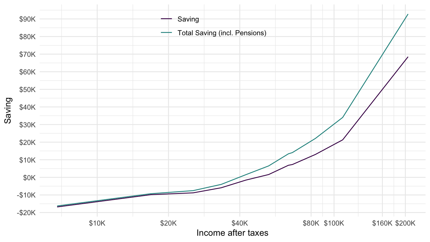
cx.series |>
  filter(demographics_code == "LB15",
         item_code %in% c("INCAFTTX", "HOUSING", "PENSIONS", "TOTALEXP", "OWNMORTG")) |>
  inner_join(cx.data.1.AllData |>
              filter(year == 2016), by = "series_id") |>
  inner_join(cx.characteristics |>
              select(1, 2, 3), by = c("characteristics_code", "demographics_code")) |>
  select(characteristics_text, item_code, value) |>
  spread(item_code, value) |>
  transmute(characteristics_text,
            INCAFTTX,
            `Saving Rate` = (INCAFTTX - TOTALEXP)/INCAFTTX,
            `Total Saving Rate (incl. Pensions)` = (INCAFTTX - TOTALEXP + PENSIONS)/INCAFTTX) |>
  gather(variable, value, -1, -2) |>
  ggplot() + geom_line(aes(x = INCAFTTX/1000, y = value, color = variable)) +
  theme_minimal() + xlab("Income after taxes") + ylab("Saving Rate") +
  theme(legend.position = c(0.65, 0.3),
        legend.title = element_blank()) +
  scale_x_log10(breaks = c(10, 20, 40, 80, 100, 160, 200),
                     labels = dollar_format(suffix = "K", accuracy = 1)) +
  scale_color_manual(values = viridis(3)[1:2]) +
  scale_y_continuous(breaks = 0.01*seq(-500, 200, 20),
                     labels = percent_format(accuracy = 1))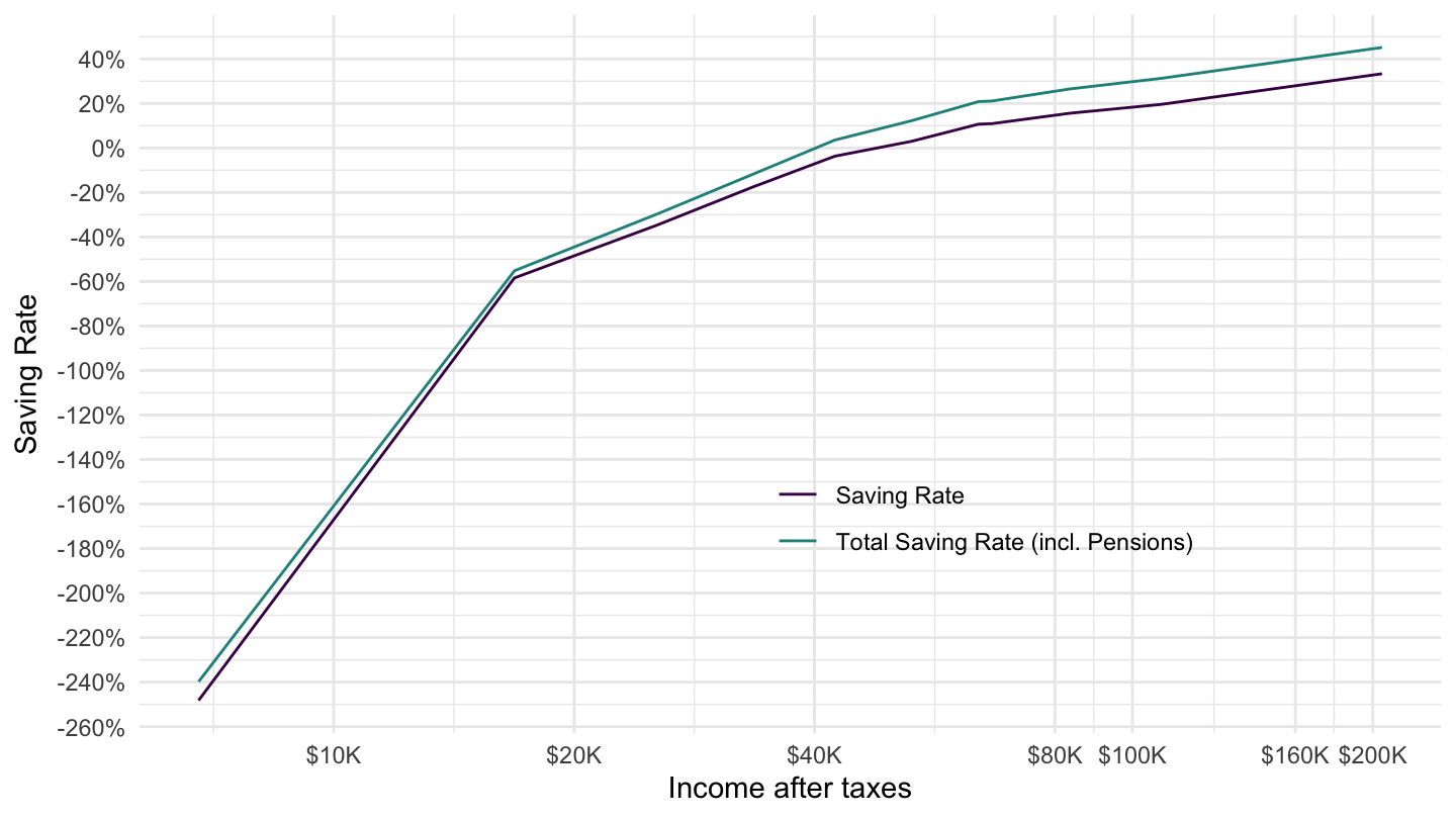
cx.series |>
  filter(demographics_code == "LB15",
         item_code %in% c("INCAFTTX", "HOUSING", "PENSIONS", "TOTALEXP", "OWNMORTG")) |>
  inner_join(cx.data.1.AllData |>
              filter(year == 2016), by = "series_id") |>
  inner_join(cx.characteristics |>
              select(1, 2, 3), by = c("characteristics_code", "demographics_code")) |>
  select(characteristics_text, item_code, value) |>
  spread(item_code, value) |>
  transmute(characteristics_text,
            INCAFTTX,
            `Saving Rate` = (INCAFTTX - TOTALEXP)/INCAFTTX,
            `Total Saving Rate (incl. Pensions)` = (INCAFTTX - TOTALEXP + PENSIONS)/INCAFTTX) |>
  gather(variable, value, -1, -2) |>
  filter(INCAFTTX > 30000) |>
  ggplot() + geom_line(aes(x = INCAFTTX/1000, y = value, color = variable)) +
  theme_minimal() + xlab("Income after taxes") + ylab("Saving Rate") +
  theme(legend.position = c(0.65, 0.3),
        legend.title = element_blank()) +
  scale_x_log10(breaks = c(10, 20, 30, 40, 50, 60, 70, 80, 100, 120, 140, 160, 200),
                     labels = dollar_format(suffix = "K", accuracy = 1)) +
  scale_color_manual(values = viridis(3)[1:2]) +
  scale_y_continuous(breaks = 0.01*seq(-500, 200, 10),
                     labels = percent_format(accuracy = 1))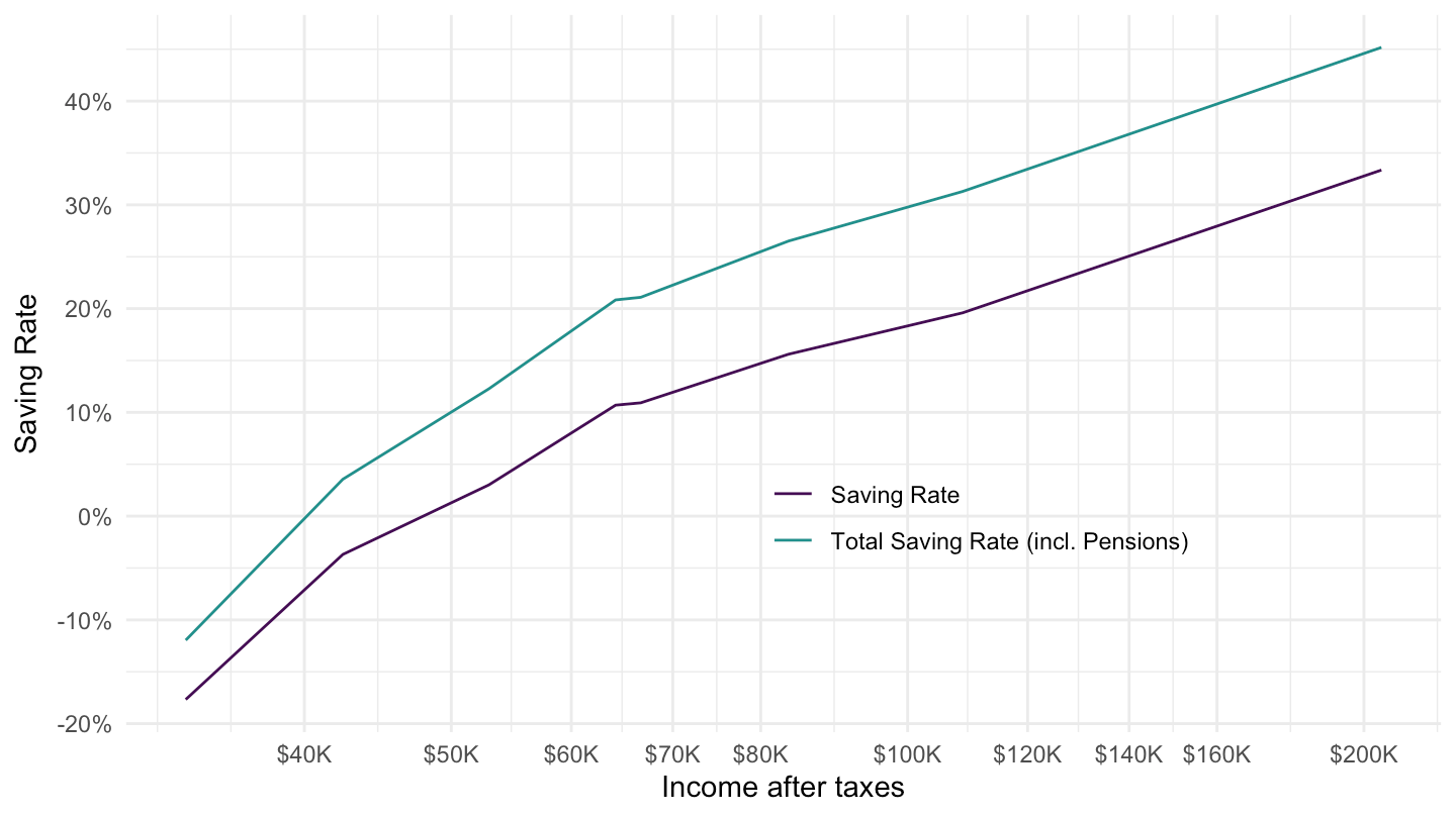
cx.series |>
  filter(demographics_code == "LB15",
         item_code %in% c("INCAFTTX", "HOUSING", "PENSIONS", "TOTALEXP", "OWNMORTG")) |>
  inner_join(cx.data.1.AllData |>
              filter(year == 2016), by = "series_id") |>
  inner_join(cx.characteristics |>
              select(1, 2, 3), by = c("characteristics_code", "demographics_code")) |>
  select(characteristics_text, item_code, value) |>
  spread(item_code, value) |>
  transmute(characteristics_text,
            INCAFTTX,
            `Total Expenditures (incl. Pensions)` = TOTALEXP,
            `Total Expenditures` = TOTALEXP - PENSIONS) |>
  gather(variable, value, -1, -2) |>
  ggplot() + geom_line(aes(x = INCAFTTX/1000, y = value/1000, color = variable)) +
  theme_minimal() + xlab("Income after taxes") + ylab("Consumption") +
  theme(legend.position = c(0.45, 0.9),
        legend.title = element_blank()) +
  scale_x_continuous(breaks = seq(0, 200, 20),
                     labels = dollar_format(suffix = "K", accuracy = 1)) +
  scale_color_manual(values = viridis(3)[1:2]) +
  scale_y_continuous(breaks = seq(-100, 200, 10),
                     labels = dollar_format(suffix = "K", accuracy = 1))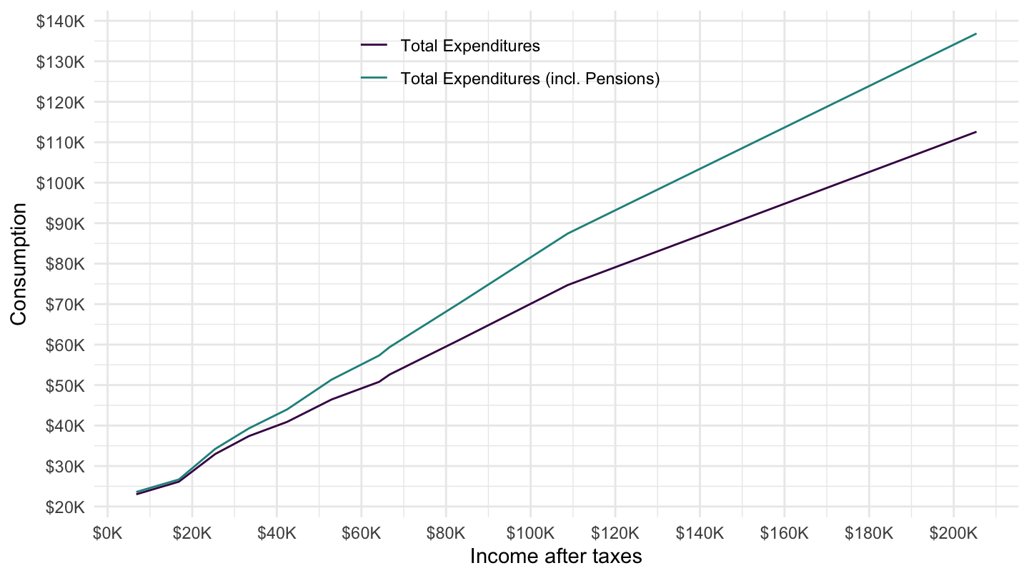
cx.series |>
  filter(demographics_code == "LB15",
         item_code %in% c("INCAFTTX", "HOUSING", "PENSIONS", "TOTALEXP", "OWNMORTG")) |>
  inner_join(cx.data.1.AllData |>
              filter(year == 2016), by = "series_id") |>
  inner_join(cx.characteristics |>
              select(1, 2, 3), by = c("characteristics_code", "demographics_code")) |>
  select(characteristics_text, item_code, value) |>
  spread(item_code, value) |>
  transmute(characteristics_text,
            INCAFTTX,
            `Consumption Rate` = (TOTALEXP)/INCAFTTX,
            `Consumption Rate (incl. Pensions)` = (TOTALEXP - PENSIONS)/INCAFTTX) |>
  gather(variable, value, -1, -2) |>
  ggplot() + geom_line(aes(x = INCAFTTX/1000, y = value, color = variable)) +
  theme_minimal() + xlab("Income after taxes") + ylab("Consumption Rate") +
  theme(legend.position = c(0.65, 0.3),
        legend.title = element_blank()) +
  scale_x_continuous(breaks = seq(0, 200, 20),
                     labels = dollar_format(suffix = "K", accuracy = 1)) +
  scale_color_manual(values = viridis(3)[1:2]) +
  scale_y_continuous(breaks = 0.01*seq(-500, 200, 20),
                     labels = percent_format(accuracy = 1))
cx.series |>
  filter(demographics_code == "LB15",
         item_code %in% c("INCAFTTX", "HOUSING", "PENSIONS", "TOTALEXP", "OWNMORTG")) |>
  inner_join(cx.data.1.AllData |>
              filter(year == 2016), by = "series_id") |>
  inner_join(cx.characteristics |>
              select(1, 2, 3), by = c("characteristics_code", "demographics_code")) |>
  select(characteristics_text, item_code, value) |>
  spread(item_code, value) |>
  transmute(characteristics_text,
            INCAFTTX,
            `Total Expenditures (incl. Pensions)` = TOTALEXP,
            `Total Expenditures` = TOTALEXP - PENSIONS) |>
  gather(variable, value, -1, -2) |>
  ggplot() + geom_line(aes(x = INCAFTTX/1000, y = value/1000, color = variable)) +
  theme_minimal() + xlab("Income after taxes") + ylab("Consumption") +
  theme(legend.position = c(0.3, 0.9),
        legend.title = element_blank()) +
  scale_x_continuous(breaks = seq(0, 200, 20),
                     labels = dollar_format(suffix = "K", accuracy = 1)) +
  scale_color_manual(values = viridis(3)[1:2]) +
  scale_y_log10(breaks = seq(-100, 200, 10),
                     labels = dollar_format(suffix = "K", accuracy = 1))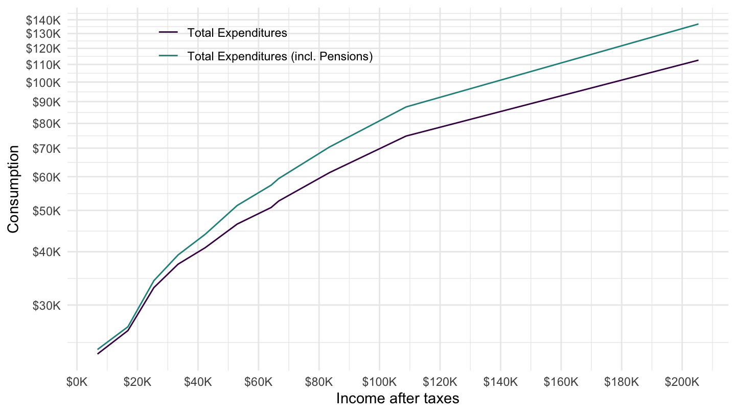
cx.series |>
  filter(demographics_code == "LB15",
         item_code %in% c("INCAFTTX", "HOUSING", "PENSIONS", "TOTALEXP", "OWNMORTG")) |>
  inner_join(cx.data.1.AllData |>
              filter(year == 2016), by = "series_id") |>
  inner_join(cx.characteristics |>
              select(1, 2, 3), by = c("characteristics_code", "demographics_code")) |>
  select(characteristics_text, item_code, value) |>
  spread(item_code, value) |>
  transmute(characteristics_text,
            INCAFTTX,
            `Consumption Rate` = (TOTALEXP)/INCAFTTX,
            `Consumption Rate (incl. Pensions)` = (TOTALEXP - PENSIONS)/INCAFTTX) |>
  gather(variable, value, -1, -2) |>
  ggplot() + geom_line(aes(x = INCAFTTX/1000, y = value, color = variable)) +
  theme_minimal() + xlab("Income after taxes") + ylab("Consumption Rate") +
  theme(legend.position = c(0.65, 0.8),
        legend.title = element_blank()) +
  scale_x_log10(breaks = c(10, 20, 40, 80, 100, 160, 200),
                     labels = dollar_format(suffix = "K", accuracy = 1)) +
  scale_color_manual(values = viridis(3)[1:2]) +
  scale_y_continuous(breaks = 0.01*seq(-500, 600, 20),
                     labels = percent_format(accuracy = 1))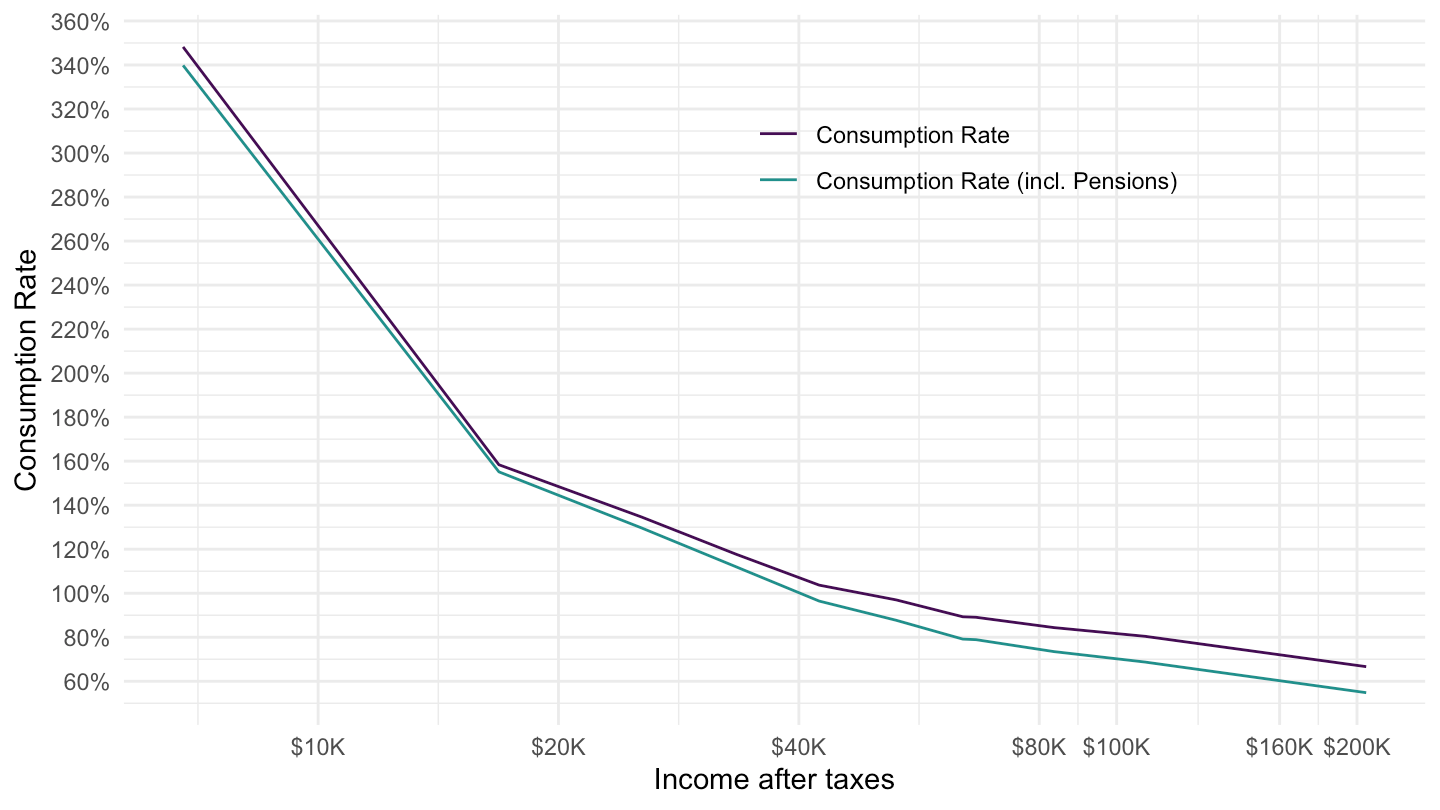
cx.series |>
  filter(demographics_code == "LB15",
         item_code %in% c("TOTALEXP", "HOUSING", "FOODTOTL", "TRANS", "INCAFTTX")) |>
  inner_join(cx.data.1.AllData |>
              filter(year == 2016), by = "series_id") |>
  inner_join(cx.characteristics |>
              select(1, 2, 3), by = c("characteristics_code", "demographics_code")) |>
  select(characteristics_text, item_code, value) |>
  spread(item_code, value) |>
  transmute(characteristics_text,
            INCAFTTX,
            `Housing (% of Expenditure)` = HOUSING/TOTALEXP,
            `Food (% of Expenditure)` = FOODTOTL/TOTALEXP,
            `Transportation (% of Expenditure)` = TRANS/TOTALEXP) |>
  gather(variable, value, -1, -2) |>
  filter(INCAFTTX > 20000) |>
  ggplot() + geom_line(aes(x = INCAFTTX/1000, y = value, color = variable)) +
  theme_minimal() + xlab("Income after taxes") + ylab("% of Expenditure") +
  theme(legend.position = c(0.65, 0.9),
        legend.title = element_blank()) +
  scale_x_continuous(breaks = seq(0, 200, 20),
                     labels = dollar_format(suffix = "K", accuracy = 1)) +
  scale_color_manual(values = viridis(4)[1:3]) +
  scale_y_continuous(breaks = 0.01*seq(-500, 200, 5),
                     labels = percent_format(accuracy = 1),
                     limits = c(0, 0.5))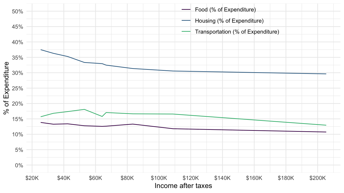
cx.series |>
  filter(demographics_code == "LB15",
         item_code %in% c("INCAFTTX", "HOUSING", "PENSIONS", "TOTALEXP", "OWNMORTG")) |>
  inner_join(cx.data.1.AllData |>
              filter(year == 2016), by = "series_id") |>
  inner_join(cx.characteristics |>
              select(1, 2, 3), by = c("characteristics_code", "demographics_code")) |>
  select(characteristics_text, item_code, value) |>
  spread(item_code, value) |>
  transmute(characteristics_text,
            INCAFTTX,
            `Housing (% of Expenditure)` = HOUSING/TOTALEXP,
            `Housing (% of Income)` = HOUSING/INCAFTTX) |>
  gather(variable, value, -1, -2) |>
  filter(INCAFTTX > 20000) |>
  ggplot() + geom_line(aes(x = INCAFTTX/1000, y = value, color = variable)) +
  theme_minimal() + xlab("Income after taxes") + ylab("Housing Consumption (%)") +
  theme(legend.position = c(0.65, 0.8),
        legend.title = element_blank()) +
  scale_x_continuous(breaks = seq(0, 200, 20),
                     labels = dollar_format(suffix = "K", accuracy = 1)) +
  scale_color_manual(values = viridis(3)[1:2]) +
  scale_y_continuous(breaks = 0.01*seq(-500, 200, 5),
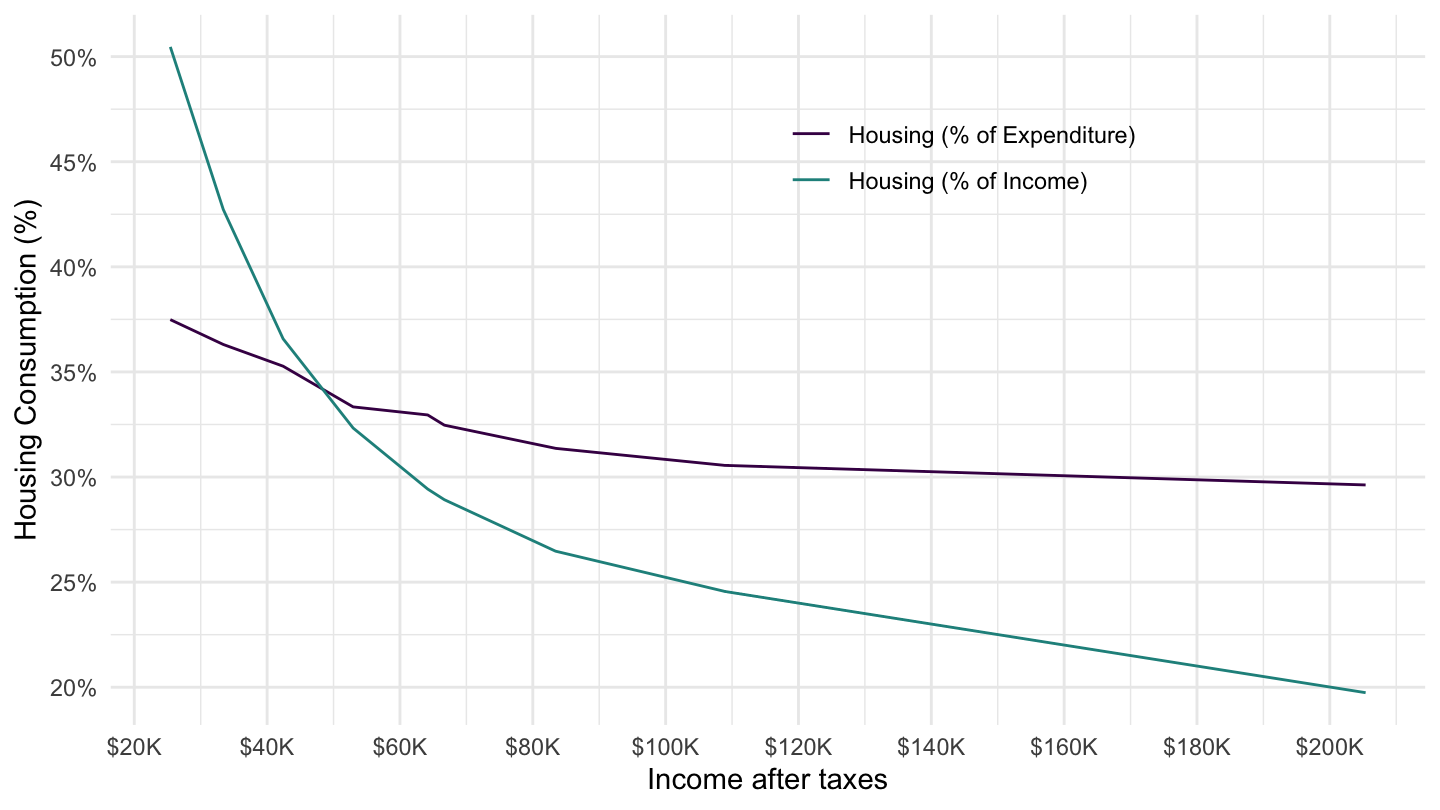
                     labels = percent_format(accuracy = 1))