Consumer Price Index - All Urban Consumers - CU

Name: Consumer Price Index - All Urban Consumers - CU
Creator: François Geerolf
License: https://www.usa.gov/government-works

Data - BLS

Author

François Geerolf

Last compile: 05 sept. 2026, 23:15

LAST_COMPILE

LAST_COMPILE
2026-09-05

Last

date	Nobs
2026-07-01	2952

List Duplicates

Figure out the structure of the data. Which is the redundant data ? It appears it’s cu.data.0.Current, cu.data.1.AllItems, cu.data.2.Summaries.

Without cu.data.0.Current (slow code - not run)

Code

new <- ls()
tibble(dataset = new) |>
  filter(grepl("cu.data", dataset),
         dataset != "cu.data.0.Current") %>%
  mutate(data = map(dataset, ~ get(.))) |>
  unnest() |>
  group_by(series_id, year, period, value, footnote_codes) |> 
  mutate(Nobs = n()) |>
  filter(Nobs > 1) |>
  arrange(series_id, year, period, value, footnote_codes)

Without cu.data.0.Current, cu.data.2.Summaries (slow code - not run)

Code

new <- ls()
tibble(dataset = new) |>
  filter(grepl("cu.data", dataset),
         dataset != "cu.data.0.Current",
         dataset != "cu.data.2.Summaries") %>%
  mutate(data = map(dataset, ~ get(.))) |>
  unnest() |>
  group_by(series_id, year, period, value, footnote_codes) |> 
  mutate(Nobs = n()) |>
  filter(Nobs > 1) |>
  arrange(series_id, year, period, value, footnote_codes)

Without cu.data.0.Current, cu.data.1.AllItems, cu.data.2.Summaries (slow code - not run)

Code

new <- ls()
tibble(dataset = new) |>
  filter(grepl("cu.data", dataset),
         dataset != "cu.data.0.Current",
         dataset != "cu.data.1.AllItems",
         dataset != "cu.data.2.Summaries") %>%
  mutate(data = map(dataset, ~ get(.))) |>
  unnest() |>
  group_by(series_id, year, period, value, footnote_codes) |> 
  mutate(Nobs = n()) |>
  filter(Nobs > 1) |>
  arrange(series_id, year, period, value, footnote_codes)

cu.series

All

Code

cu.series |>
  select(series_id, seasonal, periodicity_code, area_code, item_code,  begin_year, end_year) %>%
  {if (is_html_output()) datatable(., filter = 'top', rownames = F) else .}

Longest Series (starting before 1950)

Code

cu.series |>
  filter(begin_year <= 1950) |>
  arrange(begin_year) |>
  select(series_id, seasonal, periodicity_code, area_code, item_code,  begin_year, end_year) %>%
  {if (is_html_output()) datatable(., filter = 'top', rownames = F) else .}

cu.area

Code

cu.data |>
  left_join(cu.series, by = "series_id") |>
  left_join(cu.area, by = c("area_code")) |>
  group_by(area_code, area_name, display_level, sort_sequence) |>
  summarise(Nobs = n()) |>
  arrange(sort_sequence) %>%
  {if (is_html_output()) datatable(., filter = 'top', rownames = F) else .}

cu.item

Code

cu.data |>
  left_join(cu.series, by = "series_id") |>
  left_join(cu.item, by = c("item_code")) |>
  group_by(item_code, item_name, display_level, sort_sequence) |>
  summarise(Nobs = n()) |>
  arrange(sort_sequence) %>%
  {if (is_html_output()) datatable(., filter = 'top', rownames = F) else .}

cu.seasonal

Code

cu.data |>
  left_join(cu.series, by = "series_id") |>
  rename(seasonal_code = seasonal) |>
  left_join(cu.seasonal, by = c("seasonal_code")) |>
  group_by(seasonal_code, seasonal_text) |>
  summarise(Nobs = n()) %>%
  {if (is_html_output()) print_table(.) else .}

seasonal_code	seasonal_text	Nobs
S	Seasonally Adjusted	164034
U	Not Seasonally Adjusted	1611888

cu.periodicity

Code

cu.data |>
  left_join(cu.series, by = "series_id") |>
  left_join(cu.periodicity, by = c("periodicity_code")) |>
  group_by(periodicity_code, periodicity_name) |>
  summarise(Nobs = n()) %>%
  {if (is_html_output()) print_table(.) else .}

periodicity_code	periodicity_name	Nobs
R	Monthly	1480152
S	Semi-Annual	295770

Quality adjustments: Computers

Computers

Code

cu.data |>
  left_join(cu.series, by = "series_id") |>
  left_join(cu.item, by = "item_code") |>
  filter(series_id %in% c("CUUR0000SEEE01", "CUUR0000SEEE02")) |>
  month_to_date() |>
  group_by(series_id) |>
  mutate(value = 100*value/value[date == as.Date("1997-12-01")]) |>
  ggplot() + theme_minimal() + xlab("") + 
  ylab("Consumer Price Index") +
  geom_line(aes(x = date, y = value, color = item_name)) +
  geom_rect(data = nber_recessions |>
              filter(Trough >= as.Date("1995-01-01")), 
            aes(xmin = Peak, xmax = Trough, ymin = 0, ymax = +Inf), 
            fill = 'grey', alpha = 0.5) +
  scale_x_date(breaks = seq(1910, 2100, 2) |> paste0("-01-01") |> as.Date(),
               labels = date_format("%Y")) +
  scale_y_log10(breaks = c(10, 20, 30, 50, 80, 100, 1, 2, 3, 5, 8),
                labels = dollar_format(accuracy = 1, prefix = "")) +
  
  theme(legend.position = c(0.3, 0.2),
        legend.title = element_blank())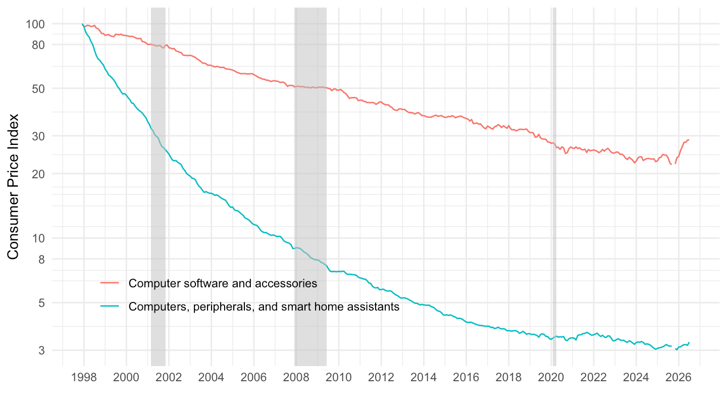

Information Technology, Hardware, Services

All

Code

cu.data |>
  left_join(cu.series, by = "series_id") |>
  left_join(cu.item, by = "item_code") |>
  filter(series_id %in% c("CUUR0000SEEE")) |>
  month_to_date() |>
  group_by(series_id) |>
  mutate(value = 100*value/value[date == as.Date("1988-12-01")]) |>
  ggplot() + theme_minimal() + xlab("") + 
  ylab("Consumer Price Index") +
  geom_line(aes(x = date, y = value, color = item_name)) +
  geom_rect(data = nber_recessions |>
              filter(Trough >= as.Date("1995-01-01")), 
            aes(xmin = Peak, xmax = Trough, ymin = 0, ymax = +Inf), 
            fill = 'grey', alpha = 0.5) +
  scale_x_date(breaks = seq(1910, 2100, 10) |> paste0("-01-01") |> as.Date(),
               labels = date_format("%Y")) +
  scale_y_log10(breaks = c(10, 20, 30, 50, 80, 100, 1, 2, 3, 5, 8),
                labels = dollar_format(accuracy = 1, prefix = "")) +
  
  theme(legend.position = c(0.3, 0.2),
        legend.title = element_blank())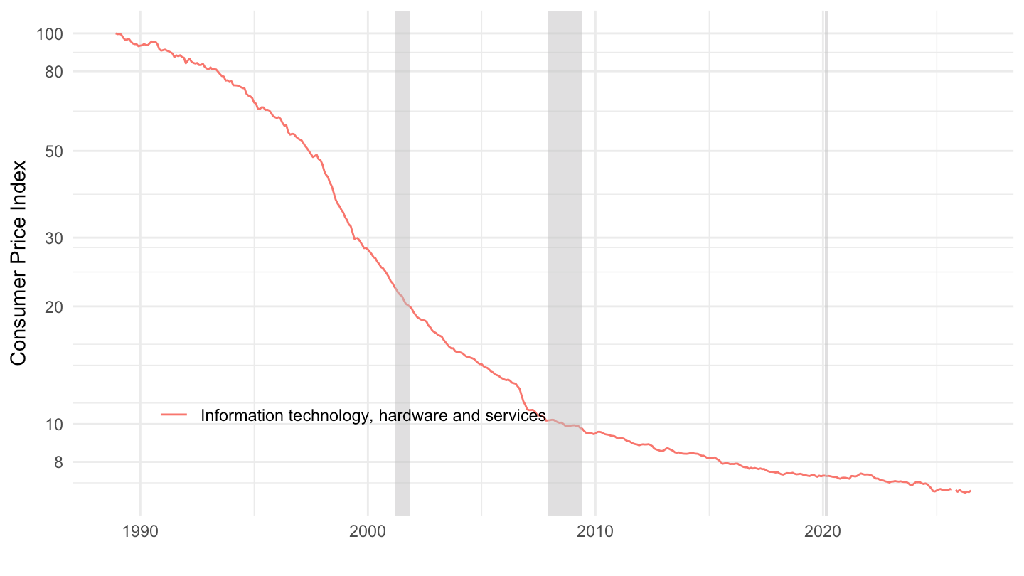

1990-

Code

cu.data |>
  left_join(cu.series, by = "series_id") |>
  left_join(cu.item, by = "item_code") |>
  filter(series_id %in% c("CUUR0000SEEE")) |>
  month_to_date() |>
  filter(date >= as.Date("1990-01-01")) |>
  group_by(series_id) |>
  mutate(value = 100*value/value[date == as.Date("1990-01-01")]) |>
  ggplot() + theme_minimal() + xlab("") + ylab("Consumer Price Index") +
  geom_line(aes(x = date, y = value, color = item_name)) +
  geom_rect(data = nber_recessions |>
              filter(Trough >= as.Date("1995-01-01")), 
            aes(xmin = Peak, xmax = Trough, ymin = 0, ymax = +Inf), 
            fill = 'grey', alpha = 0.5) +
  scale_x_date(breaks = seq(1910, 2100, 10) |> paste0("-01-01") |> as.Date(),
               labels = date_format("%Y")) +
  scale_y_log10(breaks = c(10, 20, 30, 50, 80, 100, 1, 2, 3, 5, 8),
                labels = dollar_format(accuracy = 1, prefix = "")) +
  
  theme(legend.position = c(0.3, 0.2),
        legend.title = element_blank())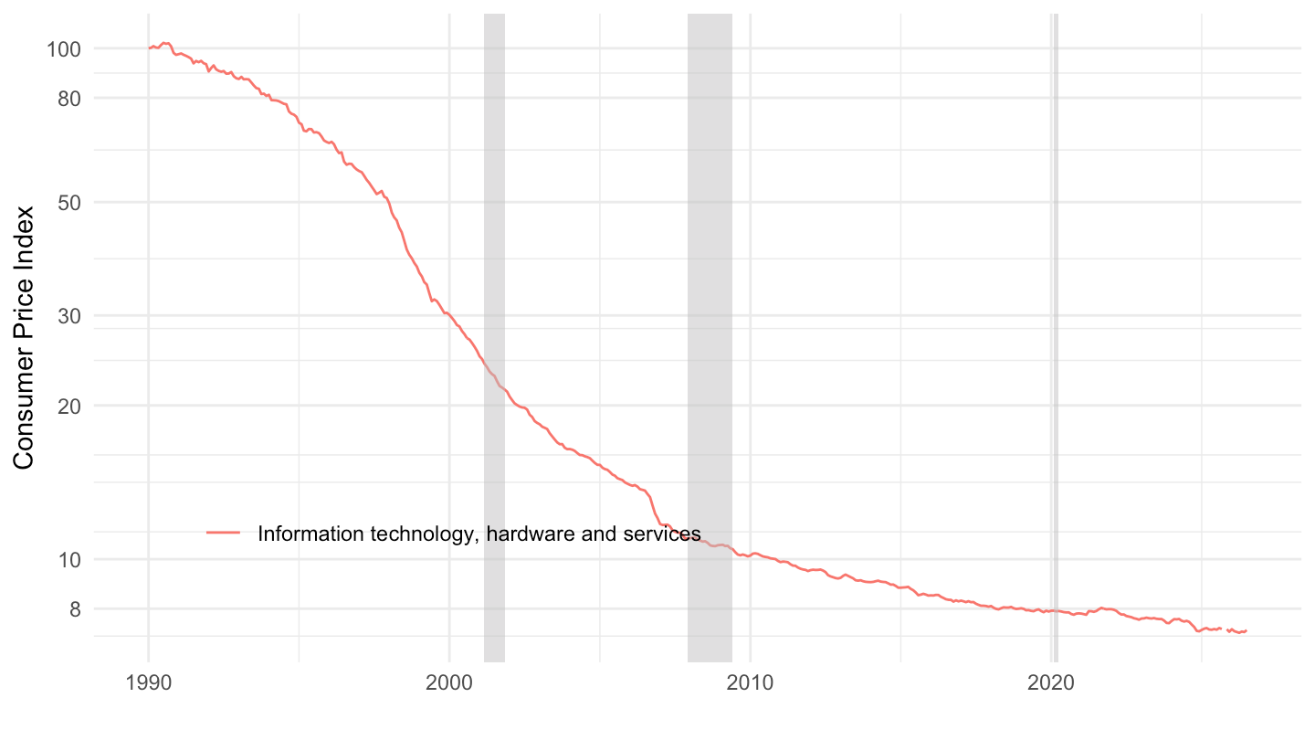

All items, Apparel, Food, Rent of primary residence

All

Code

cu.data |>
  left_join(cu.series, by = "series_id") |>
  left_join(cu.item, by = "item_code") |>
  filter(area_code == "0000",
         item_code %in% c("SA0", "SEHA", "SAA", "SAF1"),
         seasonal == "U",
         periodicity_code == "R") |>
  month_to_date() |>
  ggplot() + theme_minimal() + xlab("") + 
  ylab("Consumer Price Index") +
  geom_line(aes(x = date, y = value, color = item_name)) +
  geom_rect(data = nber_recessions |>
              filter(Trough >= as.Date("1914-01-01")), 
            aes(xmin = Peak, xmax = Trough, ymin = 0, ymax = +Inf), 
            fill = 'grey', alpha = 0.5) +
  scale_x_date(breaks = seq(1910, 2100, 10) |> paste0("-01-01") |> as.Date(),
               labels = date_format("%Y")) +
  scale_y_log10(breaks = c(seq(0, 50, 10), seq(100, 500, 50)),
                     labels = dollar_format(accuracy = 1, prefix = "")) +
  
  theme(legend.position = c(0.2, 0.80),
        legend.title = element_blank())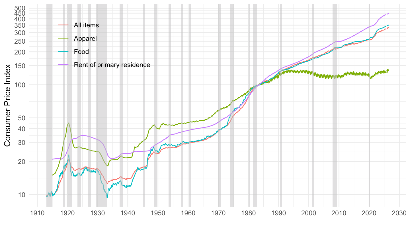

Before 1945

Code

cu.data |>
  left_join(cu.series, by = "series_id") |>
  filter(area_code == "0000",
         # SA0: All items; SEHA: All items
         item_code %in% c("SA0", "SEHA", "SAA", "SAF1"),
         seasonal == "U",
         periodicity_code == "R") |>
  left_join(cu.item, by = "item_code") |>
  month_to_date() |>
  filter(date <= as.Date("1945-01-01")) |>
  ggplot() + theme_minimal() + xlab("") + 
  ylab("Consumer Price Index") +
  geom_line(aes(x = date, y = value, color = item_name)) +
  geom_rect(data = nber_recessions |>
              filter(Peak <= as.Date("1945-01-01"),
                     Trough >= as.Date("1914-01-01")), 
            aes(xmin = Peak, xmax = Trough, ymin = 0, ymax = +Inf), 
            fill = 'grey', alpha = 0.5) +
  scale_x_date(breaks = seq(1910, 2100, 10) |> paste0("-01-01") |> as.Date(),
               labels = date_format("%Y")) +
  scale_y_log10(breaks = seq(-10, 500, 5),
                     labels = dollar_format(accuracy = 1, prefix = "")) +
  
  theme(legend.position = c(0.8, 0.9),
        legend.title = element_blank())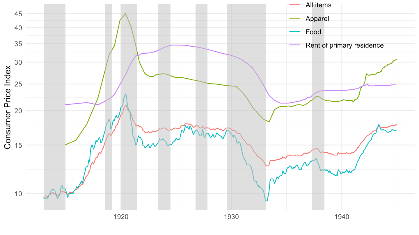

1970-1990

Code

cu.data |>
  left_join(cu.series, by = "series_id") |>
  filter(area_code == "0000",
         # SA0: All items; SEHA: All items
         item_code %in% c("SA0", "SEHA", "SAA", "SAF1"),
         seasonal == "U",
         periodicity_code == "R") |>
  left_join(cu.item, by = "item_code") |>
  month_to_date() |>
  filter(date <= as.Date("1990-01-01"),
         date >= as.Date("1970-01-01")) |>
  ggplot() + theme_minimal() + xlab("") + 
  ylab("Consumer Price Index") +
  geom_line(aes(x = date, y = value, color = item_name)) +
  geom_rect(data = nber_recessions |>
              filter(Peak <= as.Date("1990-01-01"),
                     Trough >= as.Date("1970-01-01")), 
            aes(xmin = Peak, xmax = Trough, ymin = 0, ymax = +Inf), 
            fill = 'grey', alpha = 0.5) +
  scale_x_date(breaks = seq(1910, 2100, 2) |> paste0("-01-01") |> as.Date(),
               labels = date_format("%Y")) +
  scale_y_log10(breaks = seq(-10, 500, 5),
                     labels = dollar_format(accuracy = 1, prefix = "")) +
  
  theme(legend.position = c(0.8, 0.3),
        legend.title = element_blank())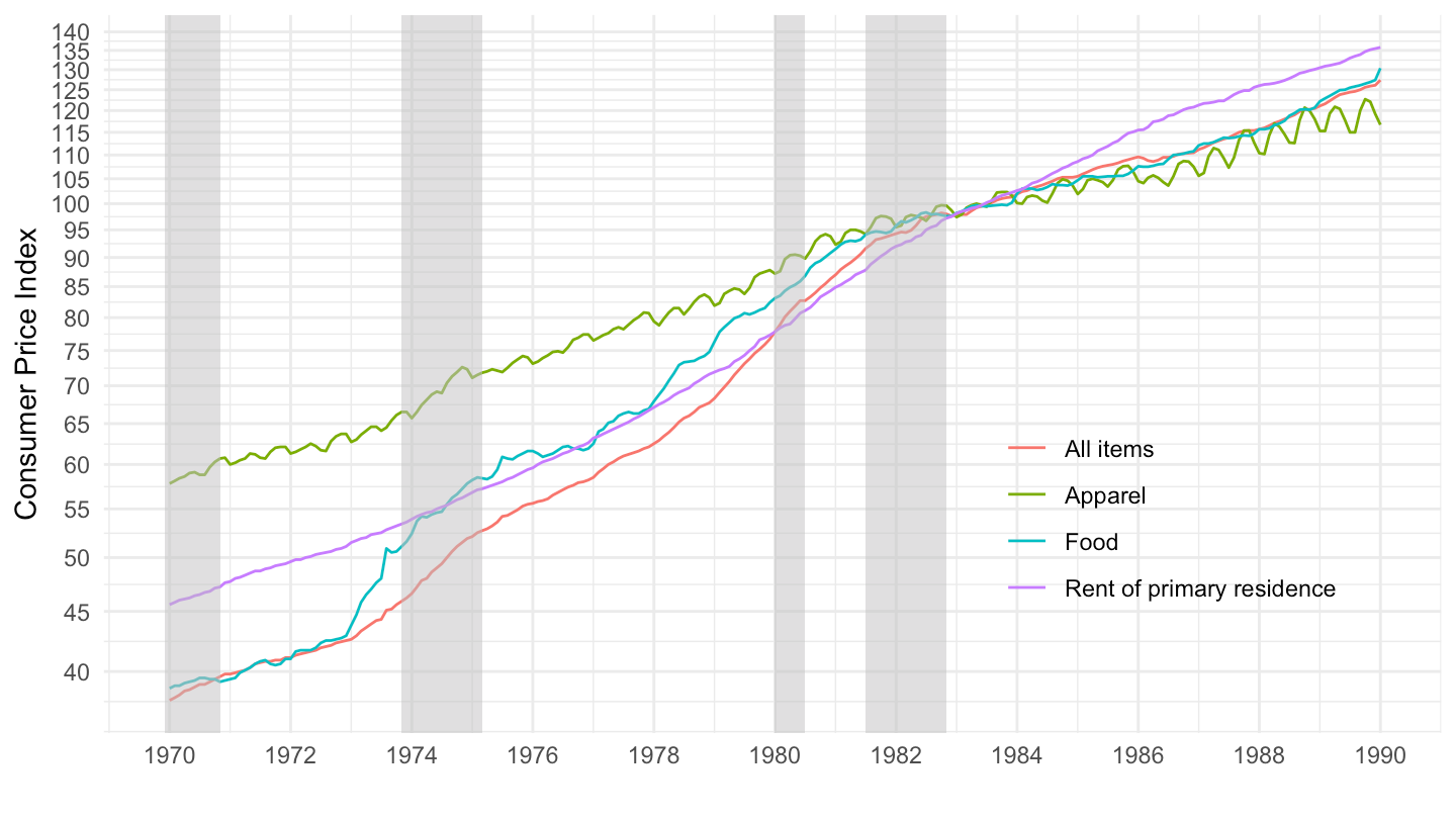

Different Components

Shelter VS All items less shelter

Code

cu.data |>
  left_join(cu.series, by = "series_id") |>
  filter(area_code == "0000",
         # SA0: All items; SEHA: All items
         item_code %in% c("SA0", "SAH1", "SA0L2"),
         seasonal == "U",
         periodicity_code == "R") |>
  month_to_date() |>
  select(date, item_code, value) |>
  spread(item_code, value) |>
  mutate(shelter_real = 100*SAH1/SA0,
         non_shelter_real = 100*SA0L2/SA0) |>
  filter(!is.na(shelter_real)) |>
  select(date, shelter_real, non_shelter_real) |>
  gather(variable, value, -date) |>
  mutate(Variable = case_when(variable == "shelter_real" ~ "Shelter",
                              variable == "non_shelter_real" ~ "All items less shelter")) |>
  ggplot() + theme_minimal() + xlab("") + ylab("Price Index (Real)") +
  geom_line(aes(x = date, y = value, color = Variable)) +
  geom_rect(data = nber_recessions |>
              filter(Trough >= as.Date("1952-01-01")), 
            aes(xmin = Peak, xmax = Trough, ymin = 0, ymax = +Inf), 
            fill = 'grey', alpha = 0.5) +
  scale_x_date(breaks = seq(1910, 2100, 5) |> paste0("-01-01") |> as.Date(),
               labels = date_format("%Y")) +
  scale_y_log10(breaks = c(seq(0, 50, 10), seq(10, 500, 10)),
                     labels = dollar_format(accuracy = 1, prefix = "")) +
  
  theme(legend.position = c(0.2, 0.80),
        legend.title = element_blank())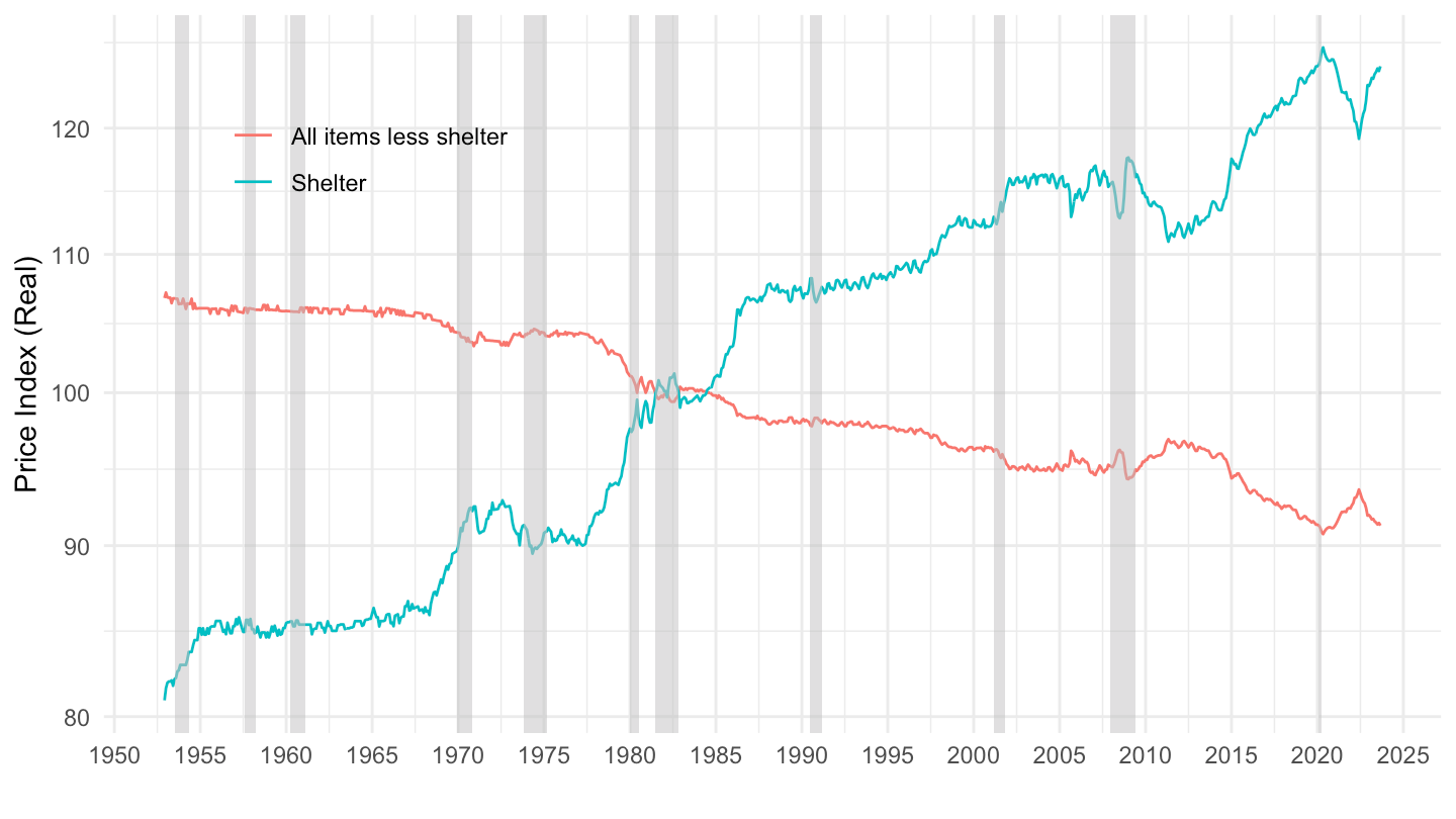

All Housing

Code

cu.data |>
  left_join(cu.series, by = "series_id") |>
  filter(area_code == "0000",
         # SA0: All items; SEHA: All items
         item_code %in% c("SA0", "SAH"),
         seasonal == "U",
         periodicity_code == "R") |>
  month_to_date() |>
  select(date, item_code, value) |>
  spread(item_code, value) |>
  mutate(rents_real = 100*SAH/SA0) |>
  filter(!is.na(rents_real)) |>
  ggplot() + theme_minimal() + xlab("") + ylab("Real Rents") +
  geom_line(aes(x = date, y = rents_real)) +
  geom_rect(data = nber_recessions |>
              filter(Trough >= as.Date("1965-01-01")), 
            aes(xmin = Peak, xmax = Trough, ymin = 0, ymax = +Inf), 
            fill = 'grey', alpha = 0.5) +
  scale_x_date(breaks = seq(1910, 2100, 5) |> paste0("-01-01") |> as.Date(),
               labels = date_format("%Y")) +
  scale_y_log10(breaks = c(seq(0, 50, 10), seq(10, 500, 2)),
                     labels = dollar_format(accuracy = 1, prefix = "")) +
  
  theme(legend.position = c(0.2, 0.80),
        legend.title = element_blank())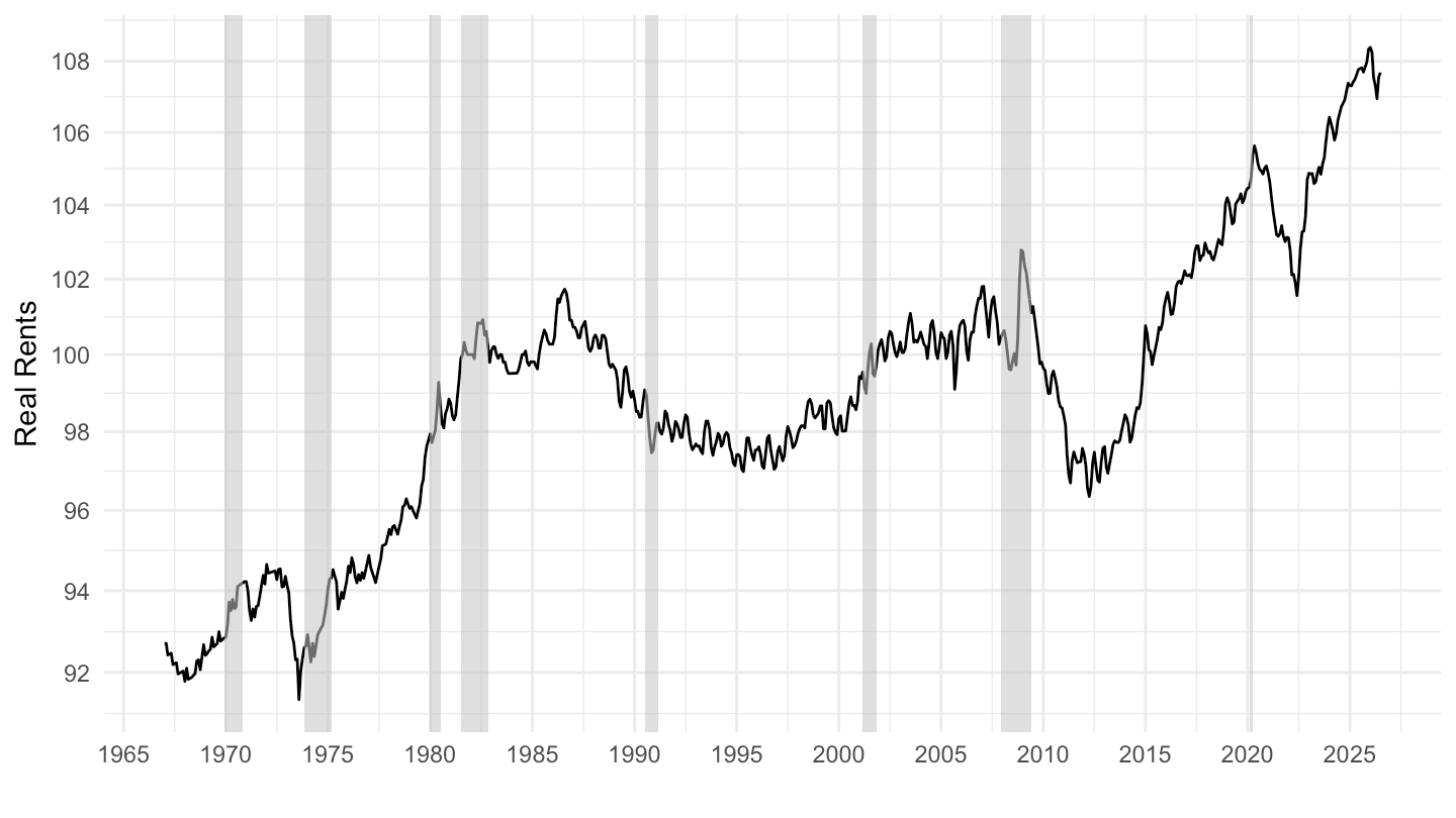

Shelter only

Code

cu.data |>
  left_join(cu.series, by = "series_id") |>
  filter(area_code == "0000",
         # SA0: All items; SEHA: All items
         item_code %in% c("SA0", "SAH1"),
         seasonal == "U",
         periodicity_code == "R") |>
  month_to_date() |>
  select(date, item_code, value) |>
  spread(item_code, value) |>
  mutate(rents_real = 100*SAH1/SA0) |>
  filter(!is.na(rents_real)) |>
  ggplot() + theme_minimal() + xlab("") + ylab("Real Rents") +
  geom_line(aes(x = date, y = rents_real)) +
  geom_rect(data = nber_recessions |>
              filter(Trough >= as.Date("1952-01-01")), 
            aes(xmin = Peak, xmax = Trough, ymin = 0, ymax = +Inf), 
            fill = 'grey', alpha = 0.5) +
  scale_x_date(breaks = seq(1910, 2100, 5) |> paste0("-01-01") |> as.Date(),
               labels = date_format("%Y")) +
  scale_y_log10(breaks = c(seq(0, 50, 10), seq(10, 500, 10)),
                     labels = dollar_format(accuracy = 1, prefix = "")) +
  
  theme(legend.position = c(0.2, 0.80),
        legend.title = element_blank())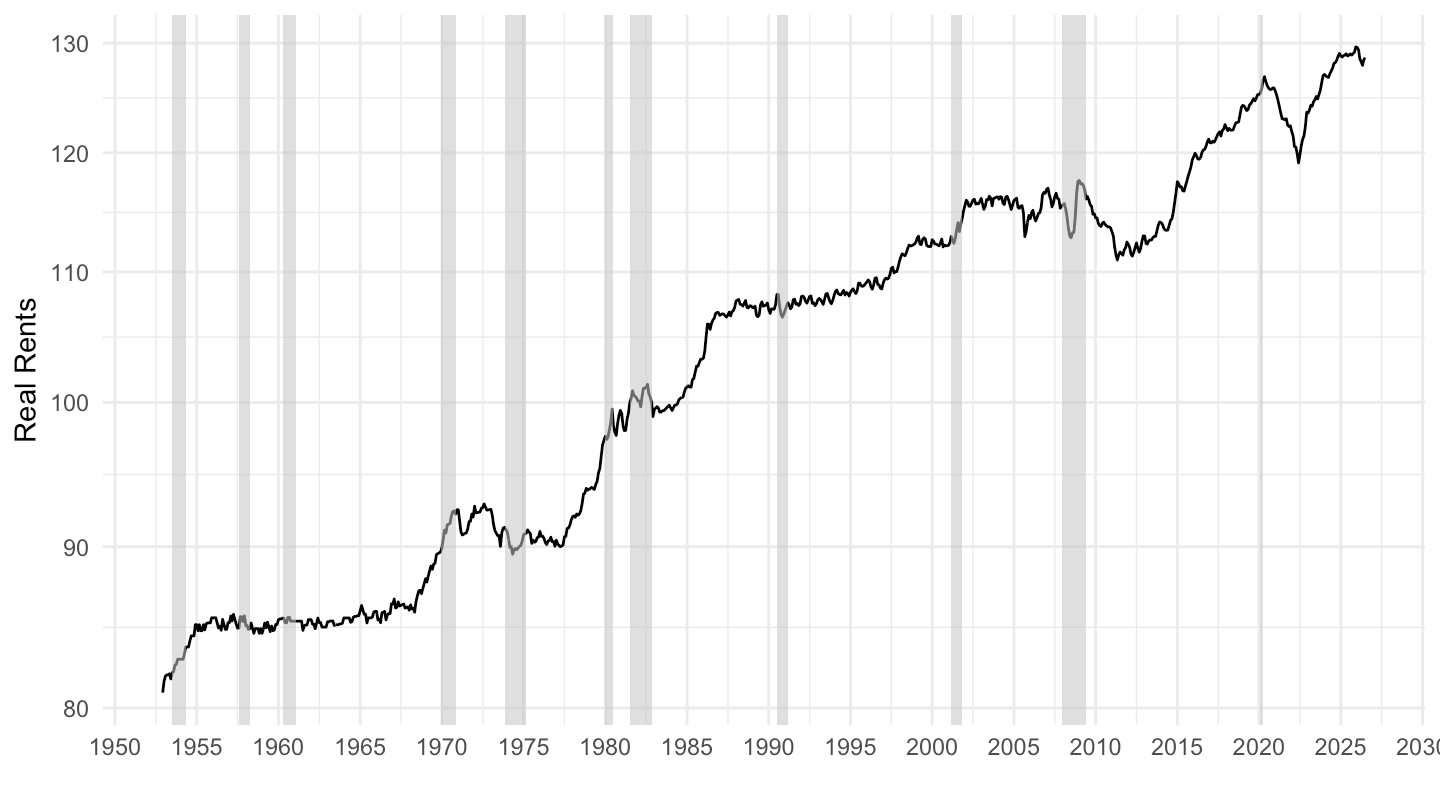

All items less shelter

Code

cu.data |>
  left_join(cu.series, by = "series_id") |>
  filter(area_code == "0000",
         # SA0: All items; SEHA: All items
         item_code %in% c("SA0", "SA0L2"),
         seasonal == "U",
         periodicity_code == "R") |>
  month_to_date() |>
  select(date, item_code, value) |>
  spread(item_code, value) |>
  mutate(rents_real = 100*SA0L2/SA0) |>
  filter(!is.na(rents_real)) |>
  ggplot() + theme_minimal() + xlab("") + ylab("All items less shelter") +
  geom_line(aes(x = date, y = rents_real)) +
  geom_rect(data = nber_recessions |>
              filter(Trough >= as.Date("1935-01-01")), 
            aes(xmin = Peak, xmax = Trough, ymin = 0, ymax = +Inf), 
            fill = 'grey', alpha = 0.5) +
  scale_x_date(breaks = seq(1910, 2100, 5) |> paste0("-01-01") |> as.Date(),
               labels = date_format("%Y")) +
  scale_y_log10(breaks = c(seq(0, 50, 10), seq(10, 500, 2)),
                     labels = dollar_format(accuracy = 1, prefix = "")) +
  
  theme(legend.position = c(0.2, 0.80),
        legend.title = element_blank())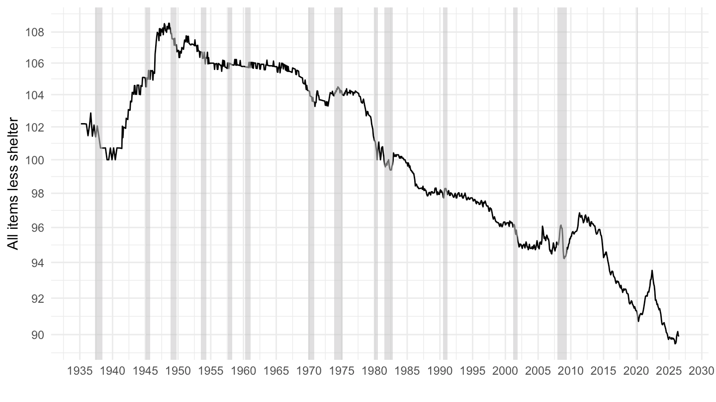

Services less rent of shelter

Code

cu.data |>
  left_join(cu.series, by = "series_id") |>
  filter(area_code == "0000",
         # SA0: All items; SEHA: All items
         item_code %in% c("SA0", "SASL2RS"),
         seasonal == "U",
         periodicity_code == "R") |>
  month_to_date() |>
  select(date, item_code, value) |>
  spread(item_code, value) |>
  mutate(rents_real = 100*SASL2RS/SA0) |>
  filter(!is.na(rents_real)) |>
  ggplot() + theme_minimal() + xlab("") + ylab("Services less rent of shelter") +
  geom_line(aes(x = date, y = rents_real)) +
  geom_rect(data = nber_recessions |>
              filter(Trough >= as.Date("1983-01-01")), 
            aes(xmin = Peak, xmax = Trough, ymin = 0, ymax = +Inf), 
            fill = 'grey', alpha = 0.5) +
  scale_x_date(breaks = seq(1910, 2100, 5) |> paste0("-01-01") |> as.Date(),
               labels = date_format("%Y")) +
  scale_y_log10(breaks = c(seq(0, 50, 10), seq(10, 500, 2)),
                     labels = dollar_format(accuracy = 1, prefix = "")) +
  
  theme(legend.position = c(0.2, 0.80),
        legend.title = element_blank())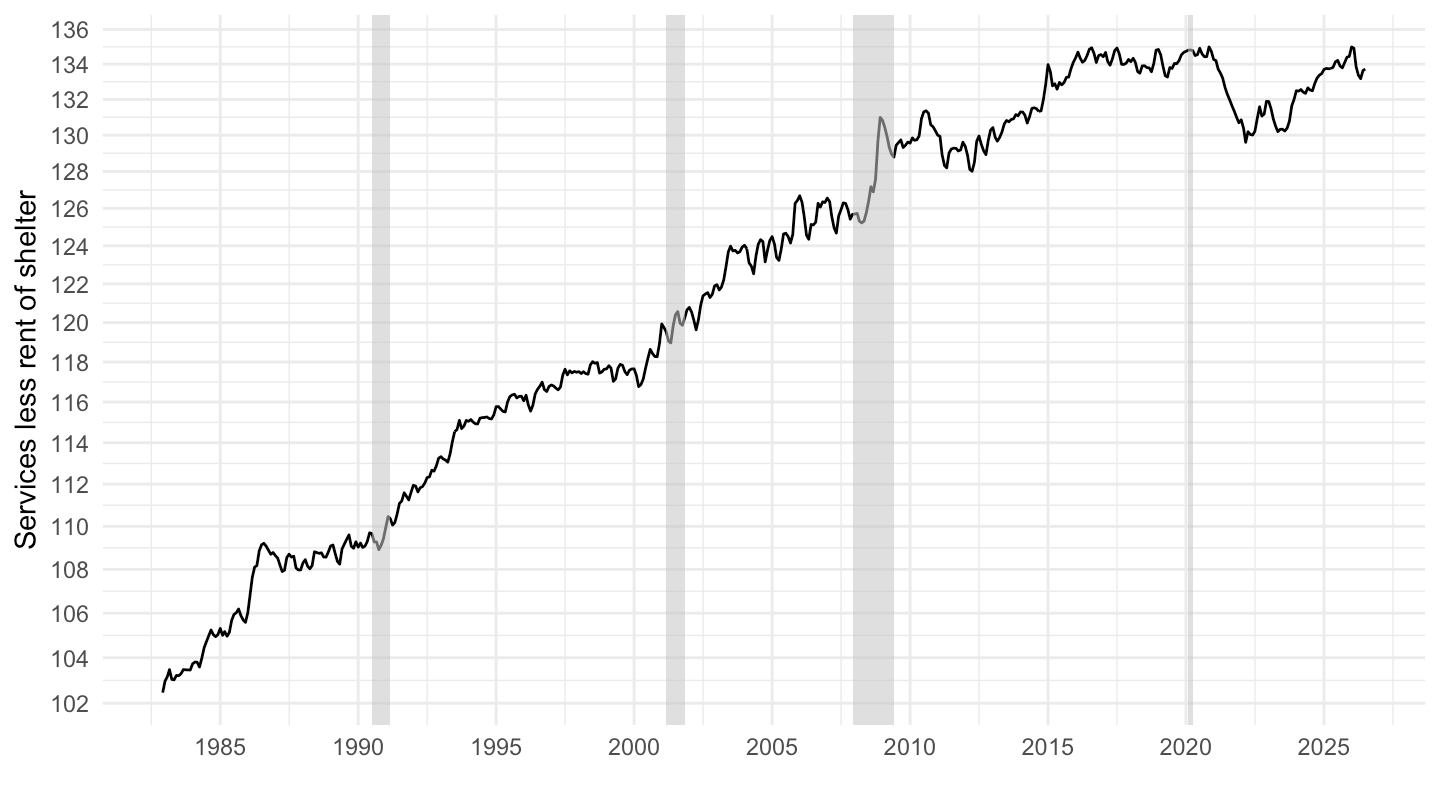

Rent of shelter

Code

cu.data |>
  left_join(cu.series, by = "series_id") |>
  filter(area_code == "0000",
         # SA0: All items; SEHA: All items
         item_code %in% c("SA0", "SAS2RS"),
         seasonal == "U",
         periodicity_code == "R") |>
  month_to_date() |>
  select(date, item_code, value) |>
  spread(item_code, value) |>
  mutate(rents_real = 100*SAS2RS/SA0) |>
  filter(!is.na(rents_real)) |>
  ggplot() + theme_minimal() + xlab("") + ylab("Real Rents") +
  geom_line(aes(x = date, y = rents_real)) +
  geom_rect(data = nber_recessions |>
              filter(Trough >= as.Date("1982-01-01")), 
            aes(xmin = Peak, xmax = Trough, ymin = 0, ymax = +Inf), 
            fill = 'grey', alpha = 0.5) +
  scale_x_date(breaks = seq(1910, 2100, 5) |> paste0("-01-01") |> as.Date(),
               labels = date_format("%Y")) +
  scale_y_log10(breaks = c(seq(0, 50, 10), seq(10, 500, 10)),
                     labels = dollar_format(accuracy = 1, prefix = "")) +
  
  theme(legend.position = c(0.2, 0.80),
        legend.title = element_blank())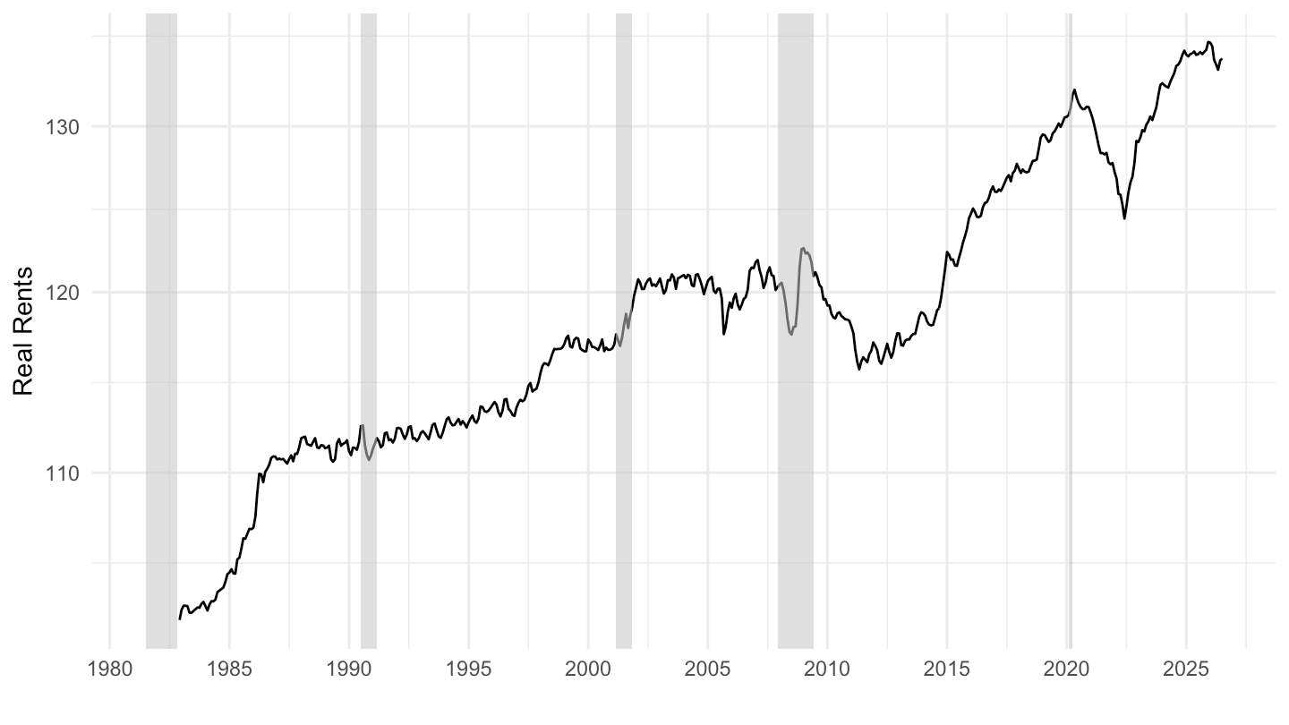

By Region, Housing including all

Heterogeneity by Area

Increase in heterogeneity ?

Code

cu.data |>
  left_join(cu.series, by = "series_id") |>
  left_join(cu.area, by = c("area_code")) |>
  filter(area_code %in% c("0100", "0200", "0300", "0400"),
         item_code %in% c("SA0", "SA0L1E"),
         seasonal == "U",
         periodicity_code == "R") |>
  month_to_date() |>
  group_by(item_code, area_code) |>
  arrange(date) |>
  filter(date >= as.Date("1996-01-01")) |>
  mutate(values = value/lag(value, 12)-1) |>
  group_by(item_code, date) |>
  summarise(values = sd(values)) |>
  ggplot() + geom_line(aes(x = date, y = values, color = item_code, linetype = item_code)) + 
  theme_minimal() + xlab("") + ylab("Standard Deviation of Regions, Unweighted (%)") +
  scale_x_date(breaks = seq(1960, 2100, 2) |> paste0("-01-01") |> as.Date(),
               labels = date_format("%Y")) +
  scale_color_manual(values = c("#1E1C1C", "#A81630")) + 
  scale_y_continuous(breaks = 0.01*seq(-20, 20, 1),
                     labels = percent_format(a = 1)) +
  theme(legend.position = c(0.55, 0.90),
        legend.title = element_blank())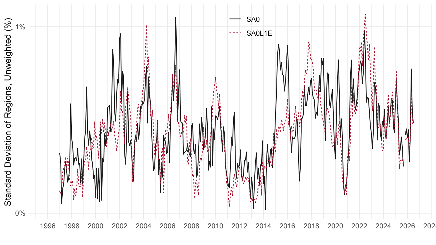

Table

Code

cu.data |>
  left_join(cu.series, by = "series_id") |>
  left_join(cu.area, by = c("area_code")) |>
  filter(# SA0: All items; SEHA: All items
         item_code %in% c("SA0"),
         seasonal == "U",
         periodicity_code == "R") |>
  month_to_date() |>
  filter(date >= as.Date("2020-02-01")) |>
  select(date, area_code, area_name, value) |>
  group_by(area_code, area_name) |>
  summarise(growth = val_near(date, value, max(date)) /
                     val_near(date, value, as.Date("2020-02-01")) - 1,
            .groups = "drop") |>
  #arrange(growth) %>%
  print_table_conditional()

Table, 2 year growth

All

Code

cu.data |>
  left_join(cu.series, by = "series_id") |>
  left_join(cu.area, by = c("area_code")) |>
  filter(# SA0: All items; SEHA: All items
         item_code %in% c("SA0"),
         seasonal == "U",
         periodicity_code == "R") |>
  month_to_date() |>
  filter(date >= as.Date("2020-02-01")) |>
  select(date, area_code, area_name, value) |>
  group_by(area_code, area_name) |>
  summarise(growth = val_near(date, value, max(date)) /
                     val_near(date, value, max(date) - 365 * 2) - 1,
            .groups = "drop") |>
  arrange(growth) |>
  print_table_conditional()

Rents

Code

cu.data |>
  left_join(cu.series, by = "series_id") |>
  left_join(cu.area, by = c("area_code")) |>
  filter(# SA0: All items; SEHA: All items
         item_code %in% c("SEHA"),
         seasonal == "U",
         periodicity_code == "R") |>
  month_to_date() |>
  filter(date >= as.Date("2020-02-01")) |>
  select(date, area_code, area_name, value) |>
  group_by(area_code, area_name) |>
  summarise(growth = val_near(date, value, max(date)) /
                     val_near(date, value, max(date) - 365 * 2) - 1,
            .groups = "drop") |>
  arrange(growth) |>
  print_table_conditional()

Std by type

Code

cu.data |>
  left_join(cu.series, by = "series_id") |>
  left_join(cu.area, by = c("area_code")) |>
  left_join(cu.item, by = c("item_code")) |>
  filter(# SA0: All items; SEHA: All items
         seasonal == "U",
         periodicity_code == "R") |>
  month_to_date() |>
  filter(date >= as.Date("2020-02-01")) |>
  select(date, area_code, area_name, item_code, item_name, value) |>
  group_by(area_code, area_name, item_code, item_name) |>
  summarise(growth = val_near(date, value, max(date)) /
                     val_near(date, value, max(date) - 365 * 2) - 1,
            .groups = "drop") |>
  ungroup() |>
  group_by(item_code, item_name) |>
  summarise(Std = sd(growth),
            Nobs = n(),
            mean = mean(growth)) |>
  arrange(-Std) |>
  filter(!is.na(Std)) |>
  print_table_conditional()

Northeast: New York, Philadelphia, Boston, Pittsburgh

Code

cu.data |>
  left_join(cu.series, by = "series_id") |>
  left_join(cu.area, by = c("area_code")) |>
  filter(area_code %in% c("S12A", "S12B", "S11A", "A104"),
         # SA0: All items; SEHA: All items
         item_code %in% c("SA0", "SEHA"),
         seasonal == "U",
         periodicity_code == "R") |>
  month_to_date() |>
  select(date, area_code, area_name, item_code, value) |>
  spread(item_code, value) |>
  mutate(rents_real = 100*SEHA/SA0) |>
  filter(!is.na(rents_real)) |>
  ggplot() + theme_minimal() + xlab("") + ylab("Real Rents") +
  geom_line(aes(x = date, y = rents_real, color = area_name)) +
  geom_rect(data = nber_recessions |>
              filter(Trough >= as.Date("1914-01-01")), 
            aes(xmin = Peak, xmax = Trough, ymin = 0, ymax = +Inf), 
            fill = 'grey', alpha = 0.5) +
  scale_x_date(breaks = seq(1910, 2100, 10) |> paste0("-01-01") |> as.Date(),
               labels = date_format("%Y")) +
  scale_y_log10(breaks = c(seq(0, 50, 10), seq(10, 500, 10)),
                     labels = dollar_format(accuracy = 1, prefix = "")) +
  
  theme(legend.position = c(0.7, 0.80),
        legend.title = element_blank())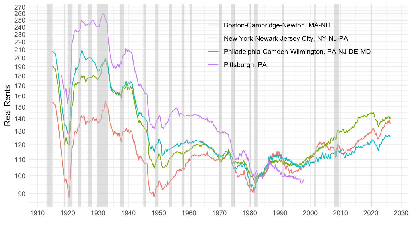

Midwest 1: Chicago, Detroit, Minneapolis, St-Louis

Code

cu.data |>
  left_join(cu.series, by = "series_id") |>
  left_join(cu.area, by = c("area_code")) |>
  filter(area_code %in% c("S23A", "S23B", "S24A", "S24B"),
         # SA0: All items; SEHA: All items
         item_code %in% c("SA0", "SEHA"),
         seasonal == "U",
         periodicity_code == "R") |>
  month_to_date() |>
  select(date, area_code, area_name, item_code, value) |>
  spread(item_code, value) |>
  mutate(rents_real = 100*SEHA/SA0) |>
  filter(!is.na(rents_real)) |>
  ggplot() + theme_minimal() + xlab("") + ylab("Real Rents") +
  geom_line(aes(x = date, y = rents_real, color = area_name)) +
  geom_rect(data = nber_recessions |>
              filter(Trough >= as.Date("1914-01-01")), 
            aes(xmin = Peak, xmax = Trough, ymin = 0, ymax = +Inf), 
            fill = 'grey', alpha = 0.5) +
  scale_x_date(breaks = seq(1910, 2100, 10) |> paste0("-01-01") |> as.Date(),
               labels = date_format("%Y")) +
  scale_y_log10(breaks = c(seq(0, 50, 10), seq(10, 500, 10)),
                     labels = dollar_format(accuracy = 1, prefix = "")) +
  
  theme(legend.position = c(0.7, 0.80),
        legend.title = element_blank())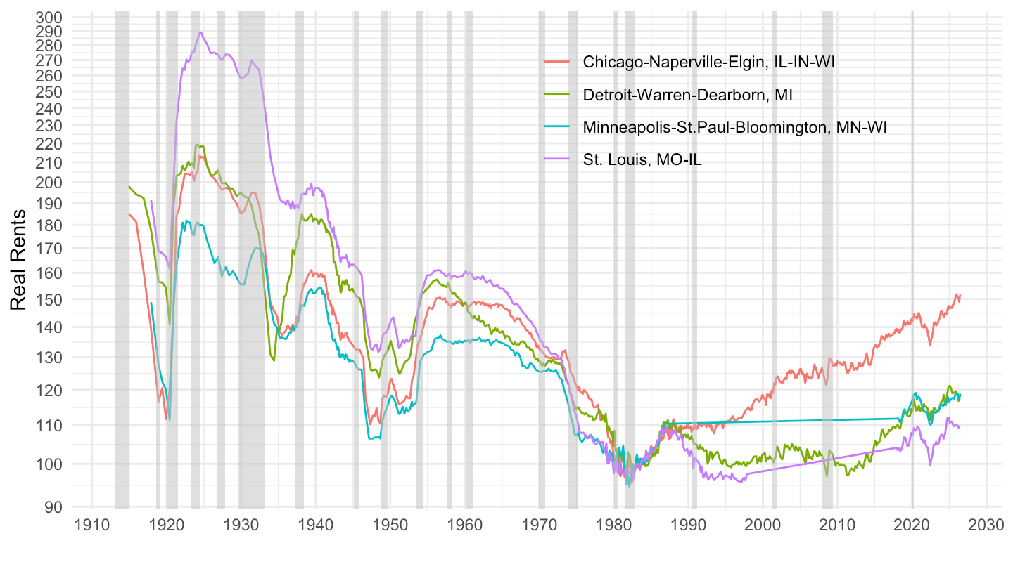

Midwest 2: Cincinnati, Cleveland, Kansas City, Milwaukee

Code

cu.data |>
  left_join(cu.series, by = "series_id") |>
  left_join(cu.area, by = c("area_code")) |>
  filter(area_code %in% c("A210", "A212", "A213", "A214"),
         # SA0: All items; SEHA: All items
         item_code %in% c("SA0", "SEHA"),
         seasonal == "U",
         periodicity_code == "R") |>
  month_to_date() |>
  select(date, area_code, area_name, item_code, value) |>
  spread(item_code, value) |>
  mutate(rents_real = 100*SEHA/SA0) |>
  filter(!is.na(rents_real)) |>
  ggplot() + theme_minimal() + xlab("") + ylab("Real Rents") +
  geom_line(aes(x = date, y = rents_real, color = area_name)) +
  geom_rect(data = nber_recessions |>
              filter(Trough >= as.Date("1914-01-01")), 
            aes(xmin = Peak, xmax = Trough, ymin = 0, ymax = +Inf), 
            fill = 'grey', alpha = 0.5) +
  scale_x_date(breaks = seq(1910, 2100, 10) |> paste0("-01-01") |> as.Date(),
               labels = date_format("%Y")) +
  scale_y_log10(breaks = c(seq(0, 50, 10), seq(10, 500, 10)),
                     labels = dollar_format(accuracy = 1, prefix = "")) +
  
  theme(legend.position = c(0.7, 0.80),
        legend.title = element_blank())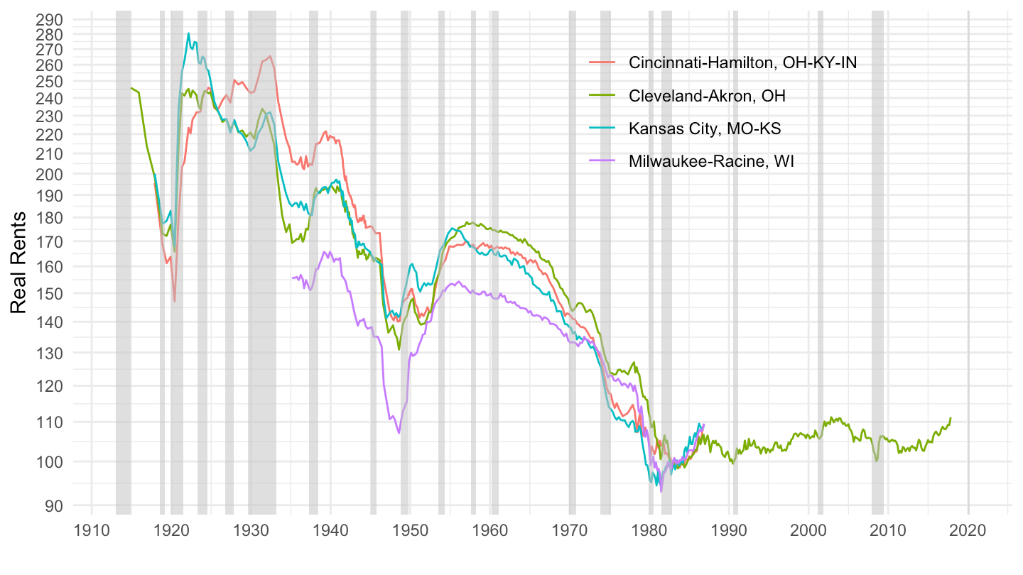

South 1: Cincinnati, Cleveland, Kansas City, Milwaukee

Code

cu.data |>
  left_join(cu.series, by = "series_id") |>
  left_join(cu.area, by = c("area_code")) |>
  filter(area_code %in% c("S35C", "S37A", "S37B", "S35B"),
         # SA0: All items; SEHA: All items
         item_code %in% c("SA0", "SEHA"),
         seasonal == "U",
         periodicity_code == "R") |>
  month_to_date() |>
  select(date, area_code, area_name, item_code, value) |>
  spread(item_code, value) |>
  mutate(rents_real = 100*SEHA/SA0) |>
  filter(!is.na(rents_real)) |>
  ggplot() + theme_minimal() + xlab("") + ylab("Real Rents") +
  geom_line(aes(x = date, y = rents_real, color = area_name)) +
  geom_rect(data = nber_recessions |>
              filter(Trough >= as.Date("1914-01-01")), 
            aes(xmin = Peak, xmax = Trough, ymin = 0, ymax = +Inf), 
            fill = 'grey', alpha = 0.5) +
  scale_x_date(breaks = seq(1910, 2100, 10) |> paste0("-01-01") |> as.Date(),
               labels = date_format("%Y")) +
  scale_y_log10(breaks = c(seq(0, 50, 10), seq(10, 500, 10)),
                     labels = dollar_format(accuracy = 1, prefix = "")) +
  
  theme(legend.position = c(0.7, 0.80),
        legend.title = element_blank())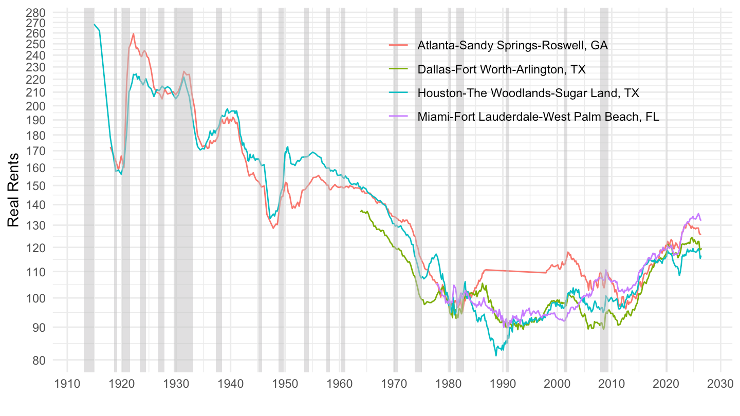

South 2: Baltimore, Tampa, Washington-Arligton, Washington-Baltimore

Code

cu.data |>
  left_join(cu.series, by = "series_id") |>
  left_join(cu.area, by = c("area_code")) |>
  filter(area_code %in% c("S35D", "S35A", "S35E", "A311"),
         # SA0: All items; SEHA: All items
         item_code %in% c("SA0", "SEHA"),
         seasonal == "U",
         periodicity_code == "R") |>
  month_to_date() |>
  select(date, area_code, area_name, item_code, value) |>
  spread(item_code, value) |>
  mutate(rents_real = 100*SEHA/SA0) |>
  filter(!is.na(rents_real)) |>
  ggplot() + theme_minimal() + xlab("") + ylab("Real Rents") +
  geom_line(aes(x = date, y = rents_real, color = area_name)) +
  scale_x_date(breaks = seq(1910, 2100, 10) |> paste0("-01-01") |> as.Date(),
               labels = date_format("%Y")) +
  scale_y_log10(breaks = c(seq(0, 50, 10), seq(10, 500, 10)),
                     labels = dollar_format(accuracy = 1, prefix = "")) +
  
  theme(legend.position = c(0.3, 0.80),
        legend.title = element_blank())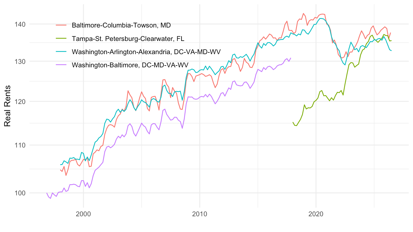

West 1: Los Angeles, Phoenix, Riverside, San diego

Code

cu.data |>
  left_join(cu.series, by = "series_id") |>
  left_join(cu.area, by = c("area_code")) |>
  filter(area_code %in% c("S49A", "S49C", "S48A", "S49E"),
         # SA0: All items; SEHA: All items
         item_code %in% c("SA0", "SEHA"),
         seasonal == "U",
         periodicity_code == "R") |>
  month_to_date() |>
  select(date, area_code, area_name, item_code, value) |>
  spread(item_code, value) |>
  mutate(rents_real = 100*SEHA/SA0) |>
  filter(!is.na(rents_real)) |>
  ggplot() + theme_minimal() + xlab("") + ylab("Real Rents") +
  geom_line(aes(x = date, y = rents_real, color = area_name)) +
  scale_x_date(breaks = seq(1910, 2100, 10) |> paste0("-01-01") |> as.Date(),
               labels = date_format("%Y")) +
  scale_y_log10(breaks = c(seq(0, 50, 10), seq(10, 500, 10)),
                     labels = dollar_format(accuracy = 1, prefix = "")) +
  
  theme(legend.position = c(0.6, 0.80),
        legend.title = element_blank())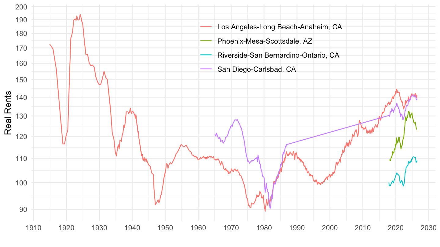

West 2: Los Angeles, Phoenix, Riverside, San diego

Code

cu.data |>
  left_join(cu.series, by = "series_id") |>
  left_join(cu.area, by = c("area_code")) |>
  filter(area_code %in% c("S49B", "S49D", "A421", "A425"),
         # SA0: All items; SEHA: All items
         item_code %in% c("SA0", "SEHA"),
         seasonal == "U",
         periodicity_code == "R") |>
  month_to_date() |>
  select(date, area_code, area_name, item_code, value) |>
  spread(item_code, value) |>
  mutate(rents_real = 100*SEHA/SA0) |>
  filter(!is.na(rents_real)) |>
  ggplot() + theme_minimal() + xlab("") + ylab("Real Rents") +
  geom_line(aes(x = date, y = rents_real, color = area_name)) +
  scale_x_date(breaks = seq(1910, 2100, 10) |> paste0("-01-01") |> as.Date(),
               labels = date_format("%Y")) +
  scale_y_log10(breaks = c(seq(0, 50, 10), seq(10, 500, 10)),
                     labels = dollar_format(accuracy = 1, prefix = "")) +
  
  theme(legend.position = c(0.6, 0.80),
        legend.title = element_blank())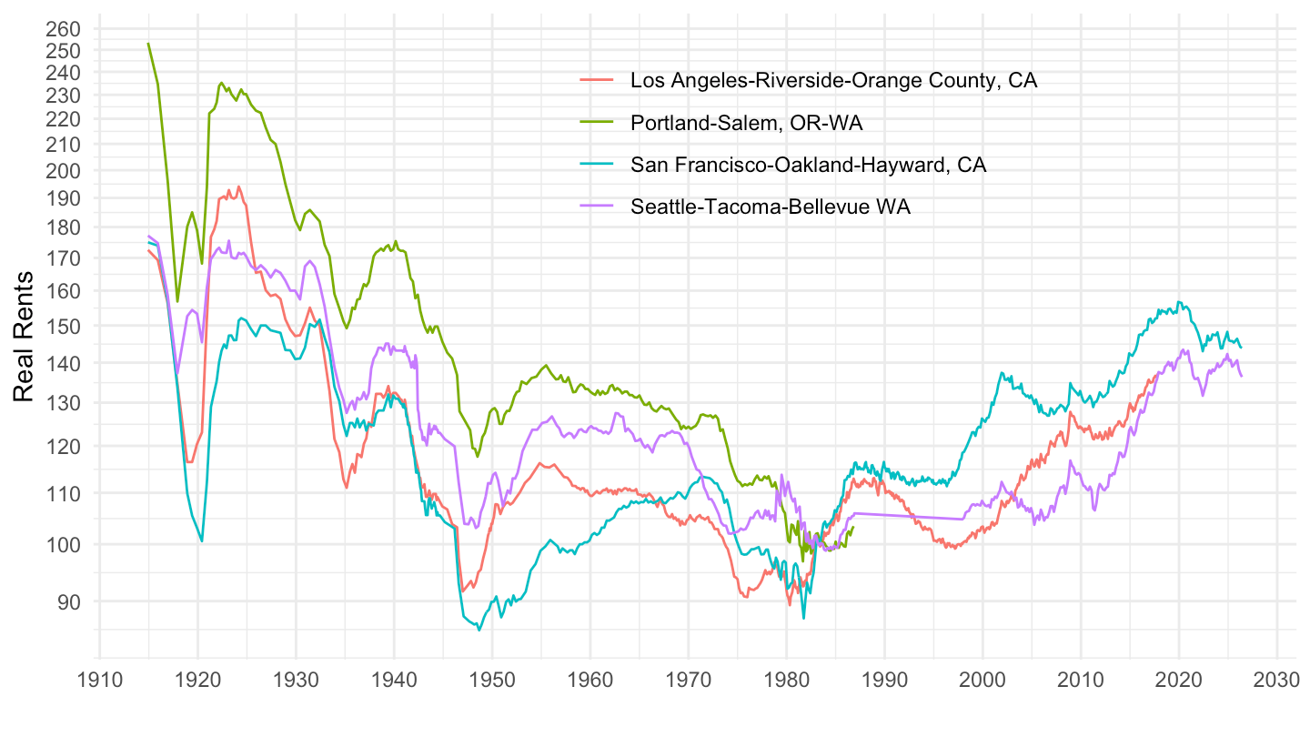

Los Angeles, New York, San Francisco

All

Code

cu.data |>
  left_join(cu.series, by = "series_id") |>
  left_join(cu.area, by = c("area_code")) |>
  filter(area_code %in% c("0000", "S12A", "S49B", "S49A"),
         # SA0: All items; SEHA: All items
         item_code %in% c("SA0", "SEHA"),
         seasonal == "U",
         periodicity_code == "R") |>
  month_to_date() |>
  select(date, area_code, area_name, item_code, value) |>
  spread(item_code, value) |>
  mutate(rents_real = 100*SEHA/SA0) |>
  filter(!is.na(rents_real)) |>
  ggplot() + theme_minimal() + xlab("") + ylab("Real Rents") +
  geom_line(aes(x = date, y = rents_real, color = area_name)) +
  geom_rect(data = nber_recessions |>
              filter(Trough >= as.Date("1914-01-01")), 
            aes(xmin = Peak, xmax = Trough, ymin = 0, ymax = +Inf), 
            fill = 'grey', alpha = 0.5) +
  scale_x_date(breaks = seq(1910, 2100, 10) |> paste0("-01-01") |> as.Date(),
               labels = date_format("%Y")) +
  scale_y_log10(breaks = c(seq(0, 50, 10), seq(10, 500, 10)),
                     labels = dollar_format(accuracy = 1, prefix = "")) +
  
  theme(legend.position = c(0.7, 0.80),
        legend.title = element_blank())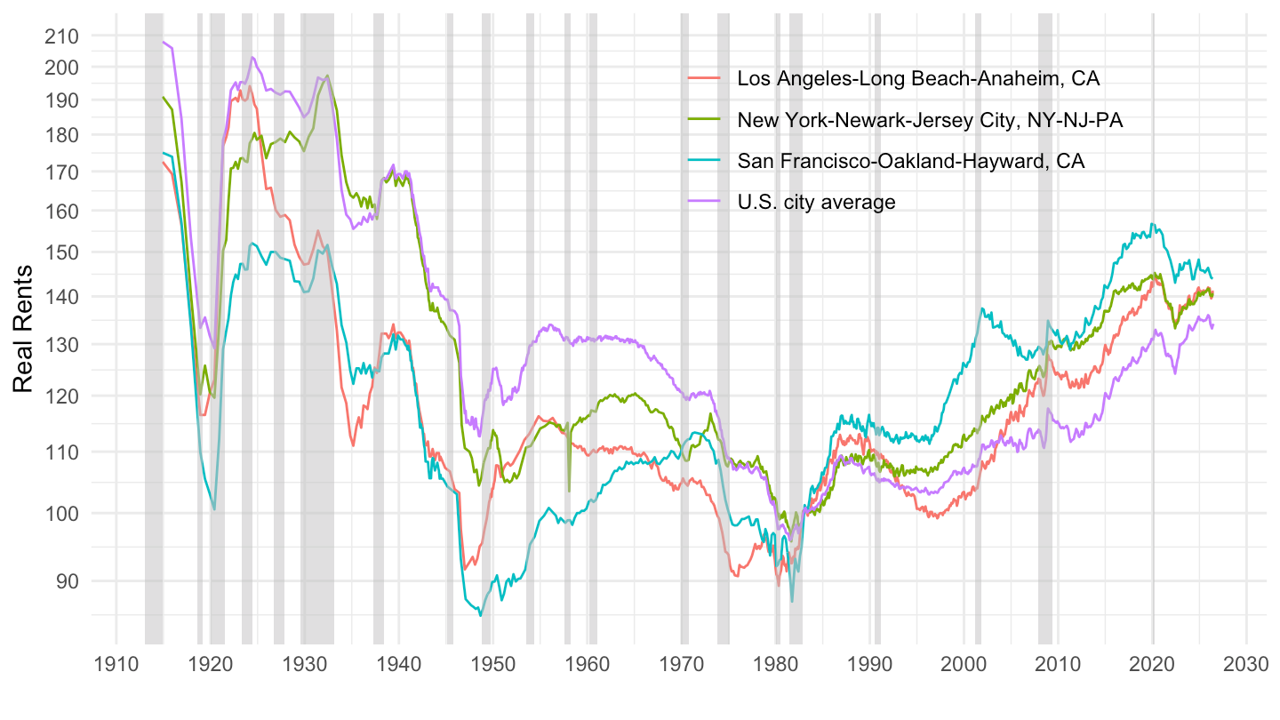

1970-

Code

cu.data |>
  left_join(cu.series, by = "series_id") |>
  left_join(cu.area, by = c("area_code")) |>
  filter(area_code %in% c("0000", "S12A", "S49B", "S49A"),
         # SA0: All items; SEHA: All items
         item_code %in% c("SA0", "SEHA"),
         seasonal == "U",
         periodicity_code == "R") |>
  month_to_date() |>
  filter(date >= as.Date("1970-01-01")) |>
  select(date, area_code, area_name, item_code, value) |>
  spread(item_code, value) |>
  mutate(rents_real = 100*SEHA/SA0) |>
  filter(!is.na(rents_real)) |>
  ggplot() + theme_minimal() + xlab("") + ylab("Real Rents") +
  geom_line(aes(x = date, y = rents_real, color = area_name)) +
  geom_rect(data = nber_recessions |>
              filter(Trough >= as.Date("1970-01-01")), 
            aes(xmin = Peak, xmax = Trough, ymin = 0, ymax = +Inf), 
            fill = 'grey', alpha = 0.5) +
  scale_x_date(breaks = seq(1910, 2100, 10) |> paste0("-01-01") |> as.Date(),
               labels = date_format("%Y")) +
  scale_y_log10(breaks = c(seq(0, 50, 10), seq(10, 500, 10)),
                     labels = dollar_format(accuracy = 1, prefix = "")) +
  
  theme(legend.position = c(0.3, 0.80),
        legend.title = element_blank())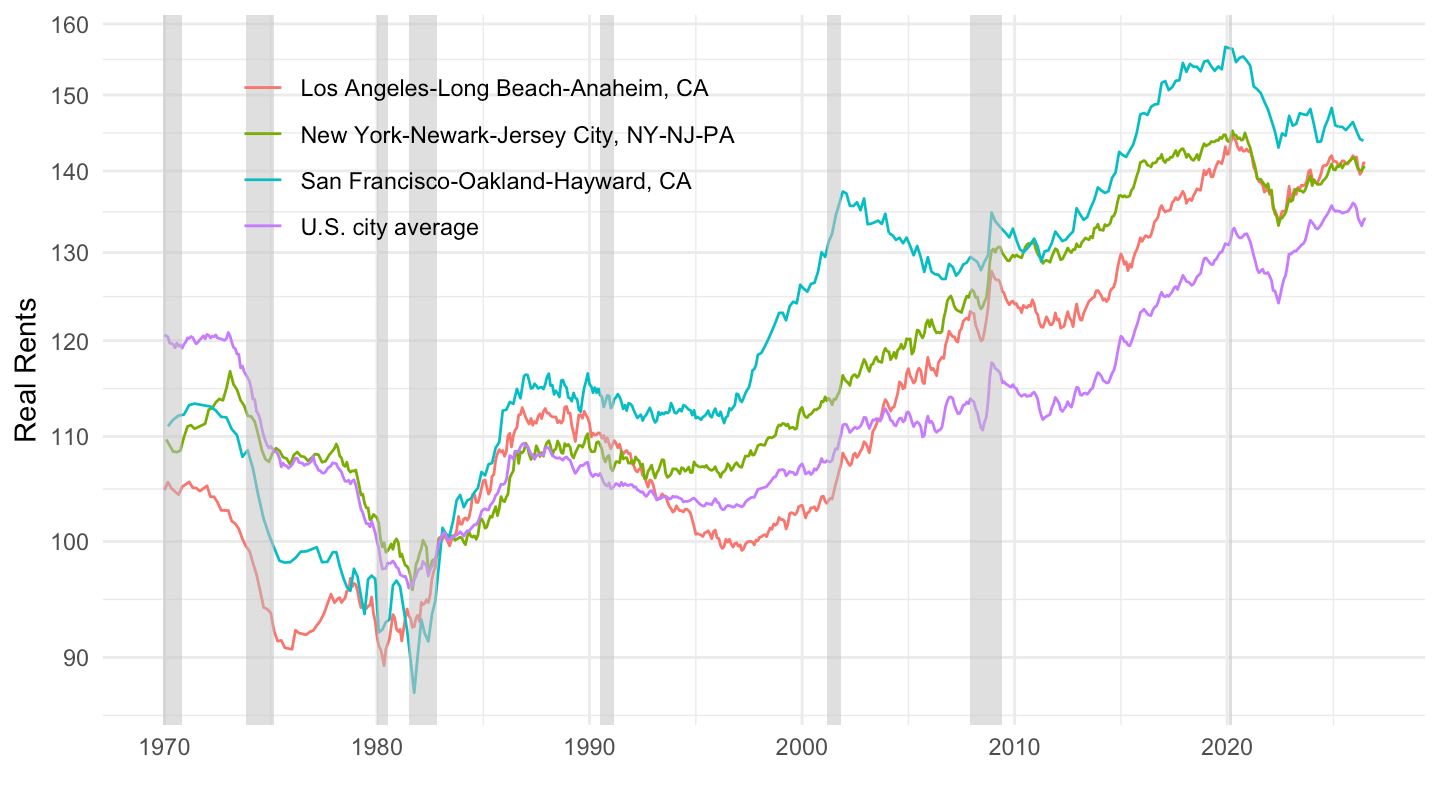

U.S. CPI

1922-1935

All

(ref:us-index-cpi) U.S. CPI (1922-1935)

Code

cu.data |>
  left_join(cu.series, by = "series_id") |>
  filter(area_code == "0000",
         item_code %in% c("SA0"),
         seasonal == "U",
         periodicity_code == "R") |>
  month_to_date() |>
  filter(date >= as.Date("1922-01-01"),
         date <= as.Date("1935-01-01"))  |> 
  ggplot() +
  geom_line(aes(x = date, y = value)) + 
  ylab("CPI") + xlab("") +
  geom_rect(data = nber_recessions, 
            aes(xmin = Peak, xmax = Trough, ymin = -Inf, ymax = +Inf), 
            fill = 'grey', alpha = 0.5) + 
  scale_y_continuous(breaks = seq(12, 18, 1),
                     limits = c(12, 18.5)) + 
  scale_x_date(breaks = as.Date(paste0(seq(1922, 1935, 1), "-01-01")),
               labels = date_format("%Y"),
               limits = c(as.Date("1922-01-01"), as.Date("1935-01-01"))) + 
  theme_minimal() + 
  geom_vline(xintercept = as.Date("1929-10-29"), linetype = "dashed", color = viridis(3)[2])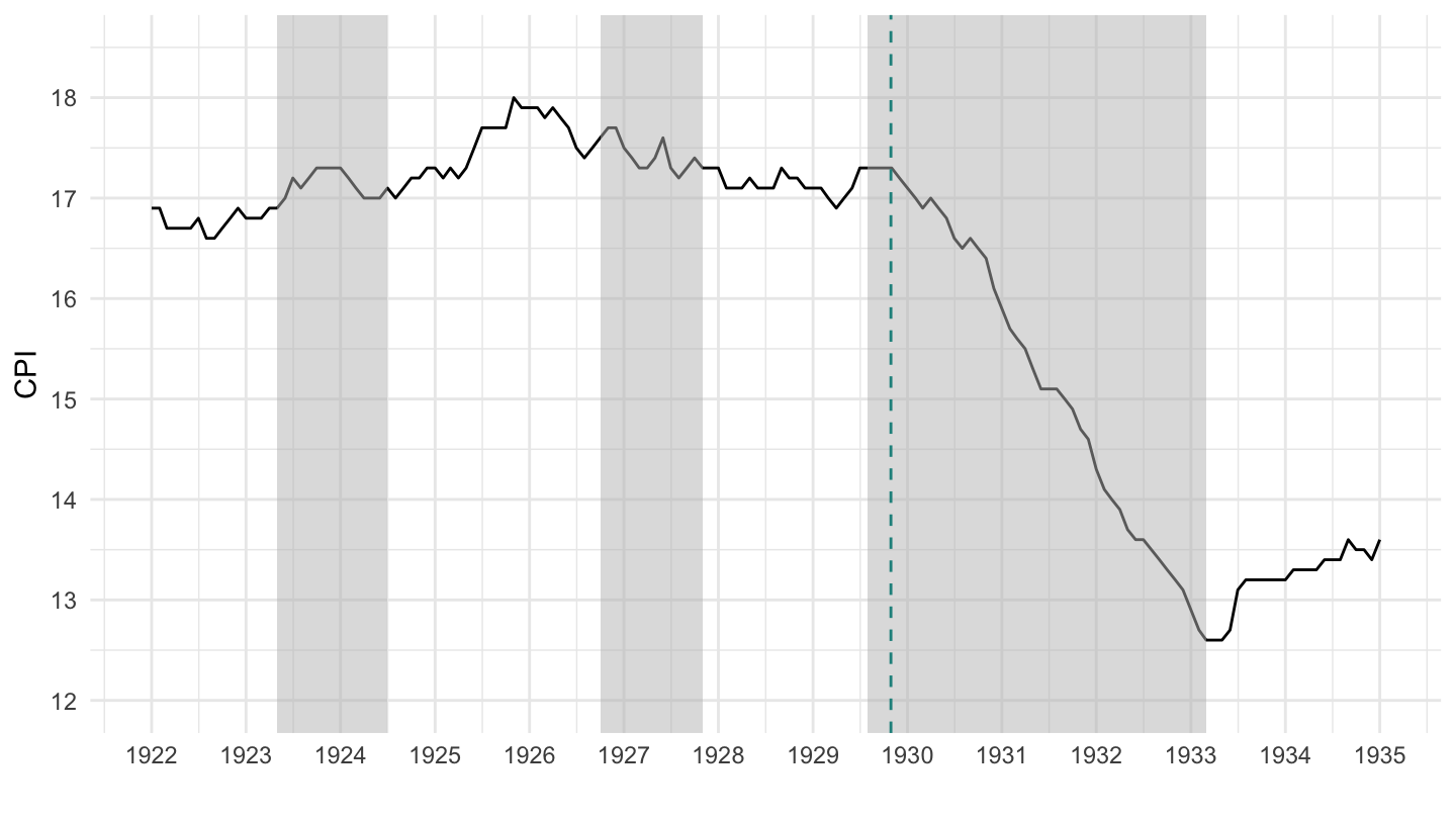

Food

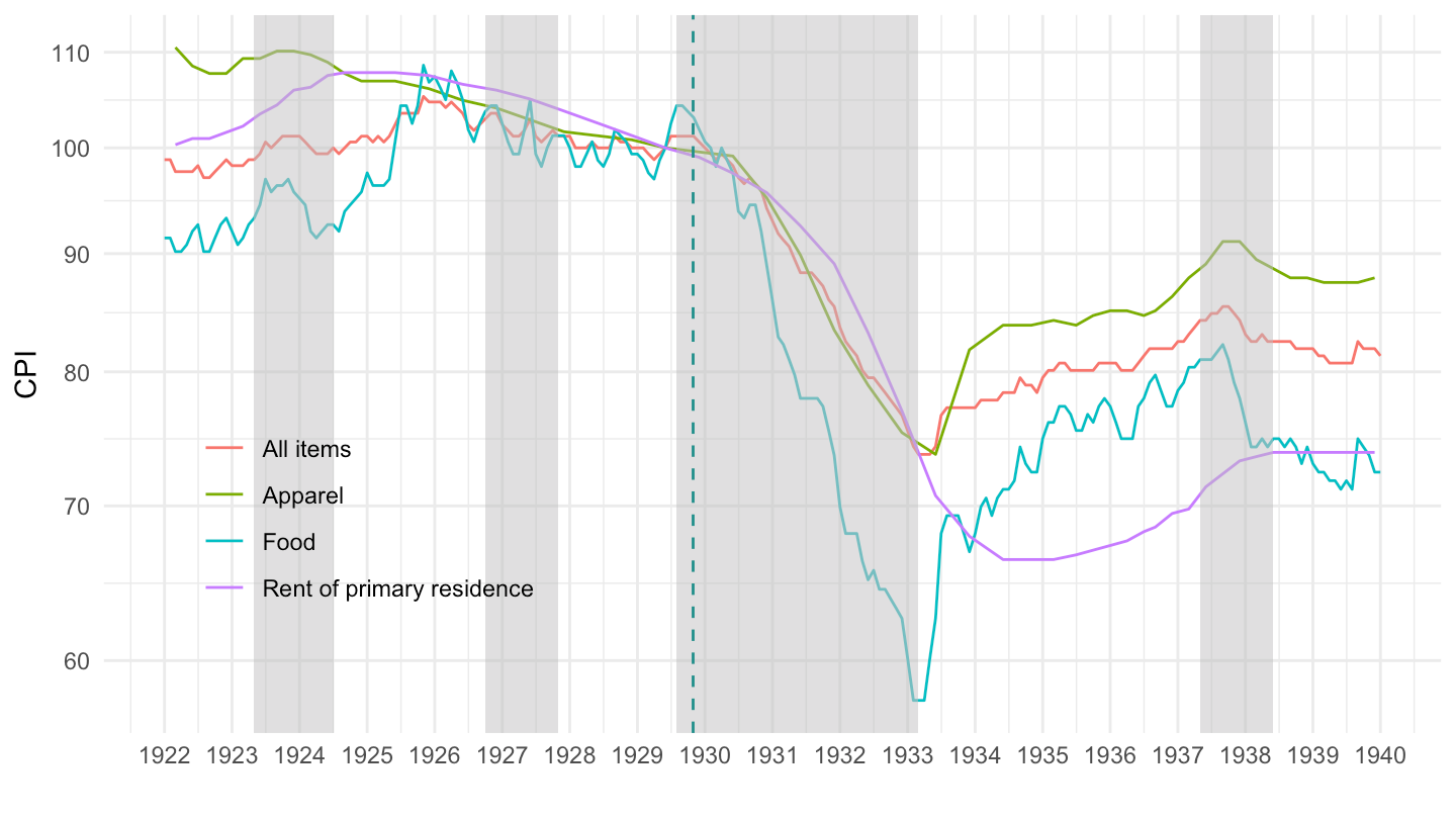
(ref:us-index-cpi-detail) U.S. CPI (1922-1935)

Code

cu.data |>
  left_join(cu.series, by = "series_id") |>
  left_join(cu.item, by = "item_code") |>
  filter(area_code == "0000",
         item_code %in% c("SA0", "SEHA", "SAA", "SAF1"),
         seasonal == "U",
         periodicity_code == "R") |>
  month_to_date() |>
  group_by(item_name) |>
  mutate(value = 100*value/value[date == as.Date("1929-06-01")]) |>
  filter(date >= as.Date("1922-01-01"),
         date <= as.Date("1940-01-01"))  |> 
  ggplot() +
  geom_line(aes(x = date, y = value, color = item_name)) +
  ylab("CPI") + xlab("") +
  geom_rect(data = nber_recessions, 
            aes(xmin = Peak, xmax = Trough, ymin = 0, ymax = +Inf), 
            fill = 'grey', alpha = 0.5) + 
  scale_y_log10(breaks = seq(10, 300, 10)) + 
  scale_x_date(breaks = as.Date(paste0(seq(1922, 1940, 1), "-01-01")),
               labels = date_format("%Y"),
               limits = c(as.Date("1922-01-01"), as.Date("1940-01-01"))) + 
  theme_minimal() + 
  geom_vline(xintercept = as.Date("1929-10-29"), linetype = "dashed", color = viridis(3)[2]) +
  
  theme(legend.position = c(0.2, 0.3),
        legend.title = element_blank())