Average Price - AP

Data - BLS

Last compile: 05 sept. 2026, 01:25

LAST_COMPILE

LAST_COMPILE
2026-09-05

Last

date	Nobs
2022-04-01	521

List Duplicates

• Without ap.data.0.Current (slow code - not run)

new <- ls()
tibble(dataset = new) |>
  filter(grepl("ap.data", dataset),
         dataset != "ap.data.0.Current") %>%
  mutate(data = map(dataset, ~ get(.))) |>
  unnest() |>
  group_by(series_id, year, period, value, footnote_codes) |> 
  mutate(Nobs = n()) |>
  filter(Nobs > 1) |>
  arrange(series_id, year, period, value, footnote_codes)

ap.item

ap.data |>
  left_join(ap.series, by = "series_id") |>
  left_join(ap.item, by = "item_code") |>
  group_by(item_code, item_name) |>
  summarise(Nobs = n()) %>%
  {if (is_html_output()) datatable(., filter = 'top', rownames = F) else .}

ap.area

ap.data |>
  left_join(ap.series, by = "series_id") |>
  left_join(ap.area, by = "area_code") |>
  group_by(area_code, area_name) |>
  summarise(Nobs = n()) %>%
  {if (is_html_output()) datatable(., filter = 'top', rownames = F) else .}

ap.series

ap.data |>
  left_join(ap.series, by = "series_id") |>
  group_by(series_id, series_title) |>
  summarise(Nobs = n()) %>%
  {if (is_html_output()) datatable(., filter = 'top', rownames = F) else .}

Ukraine

February 2022-

date0 <- as.Date("2022-02-01")
date1 <- as.Date("2022-04-01")
ap.data |>
  left_join(ap.series, by = "series_id") |>
  filter(area_code == "0000") |>
  month_to_date() |>
  filter(date %in% c(date0, date1)) |>
  left_join(ap.item, by = "item_code") |>
  group_by(item_code, item_name) |>
  filter(n() == 2) |>
  select(item_code, date, item_name, value) |>
  summarise(`February 2022` = value[date == date0],
            `Last` = value[date == date1],
            `Growth` = round(100*(value[date == date1]/value[date == date0]-1), 2)) |>
  arrange(-Growth) |>
  print_table_conditional()

September 2021-

date0 <- as.Date("2021-09-01")
date1 <- as.Date("2022-04-01")
ap.data |>
  left_join(ap.series, by = "series_id") |>
  filter(area_code == "0000") |>
  month_to_date() |>
  filter(date %in% c(date0, date1)) |>
  left_join(ap.item, by = "item_code") |>
  group_by(item_code, item_name) |>
  filter(n() == 2) |>
  select(item_code, date, item_name, value) |>
  summarise(`September 2021` = value[date == date0],
            `Last` = value[date == date1],
            `Growth` = round(100*(value[date == date1]/value[date == date0]-1), 2)) |>
  arrange(-Growth) |>
  print_table_conditional()

Gasoline price

Table - Heterogeneity

ap.data |>
  left_join(ap.series, by = "series_id") |>
  left_join(ap.item, by = "item_code") |>
  left_join(ap.area, by = "area_code") |>
  month_to_date() |>
  filter(item_code %in% c("74714"),
         date %in% as.Date(c("2015-07-01", "2018-07-01", "2019-03-01"))) |>
  select(date, area_code, area_name, value) |>
  spread(date,value) %>%
  {if (is_html_output()) datatable(., filter = 'top', rownames = F) else .}

Formulas

ap.data |>
  left_join(ap.series, by = "series_id") |>
  left_join(ap.item, by = "item_code") |>
  filter(area_code == "0000",
         item_code %in% c("74714", "7471A")) |>
  month_to_date() |>
  ggplot() + theme_minimal() + xlab("") + ylab("Price per gallon") +
  geom_line(aes(x = date, y = value, color = item_name)) +
  scale_color_manual(values = viridis(3)[1:2]) +
  geom_rect(data = nber_recessions |>
              filter(Peak > as.Date("1976-01-01")), 
            aes(xmin = Peak, xmax = Trough, ymin = -Inf, ymax = +Inf), 
            fill = 'grey', alpha = 0.5) +
  theme(legend.title = element_blank(),
        legend.position = c(0.3, 0.8)) +
  scale_y_continuous(breaks = seq(0, 6, 0.5),
                labels = scales::dollar_format(accuracy = .1)) + 
  scale_x_date(breaks = as.Date(paste0(seq(1945, 2025, 5), "-01-01")),
               labels = date_format("%Y"))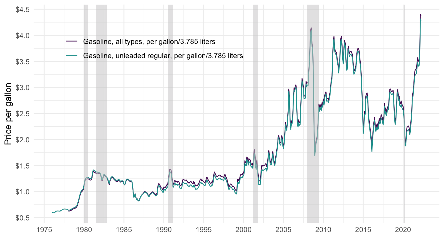

Chicago, Dallas, New York, San Francisco

All

ap.data |>
  left_join(ap.series, by = "series_id") |>
  left_join(ap.item, by = "item_code") |>
  left_join(ap.area, by = "area_code") |>
  filter(item_code %in% c("74714"),
         area_code %in% c("S49B", "S37A", "S23A", "S12A")) |>
  month_to_date() |>
  ggplot() + theme_minimal() + xlab("") + ylab("Price per gallon") +
  geom_line(aes(x = date, y = value, color = area_name)) +
  scale_color_manual(values = viridis(5)[1:4]) +
  geom_rect(data = nber_recessions |>
              filter(Peak > as.Date("1976-01-01")), 
            aes(xmin = Peak, xmax = Trough, ymin = -Inf, ymax = +Inf), 
            fill = 'grey', alpha = 0.5) +
  theme(legend.title = element_blank(),
        legend.position = c(0.3, 0.8)) +
  scale_y_log10(breaks = seq(0, 6, 0.5),
                labels = scales::dollar_format(accuracy = .1)) + 
  scale_x_date(breaks = as.Date(paste0(seq(1945, 2025, 5), "-01-01")),
               labels = date_format("%Y"))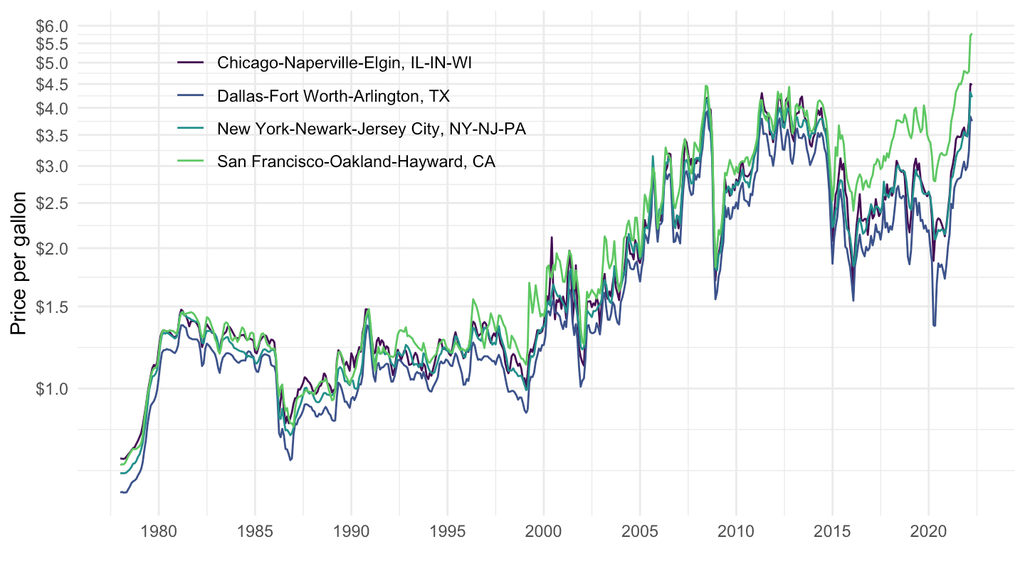

2007 -

ap.data |>
  left_join(ap.series, by = "series_id") |>
  left_join(ap.item, by = "item_code") |>
  left_join(ap.area, by = "area_code") |>
  filter(item_code %in% c("74714"),
         area_code %in% c("S49B", "S37A", "S23A", "S12A")) |>
  month_to_date() |>
  filter(date >= as.Date("2007-01-01")) |>
  ggplot() + theme_minimal() + xlab("") + ylab("Price per gallon") +
  geom_line(aes(x = date, y = value, color = area_name)) +
  scale_color_manual(values = viridis(5)[1:4]) +
  geom_rect(data = nber_recessions |>
              filter(Peak > as.Date("2007-01-01")), 
            aes(xmin = Peak, xmax = Trough, ymin = -Inf, ymax = +Inf), 
            fill = 'grey', alpha = 0.5) +
  theme(legend.title = element_blank(),
        legend.position = c(0.7, 0.85)) +
  scale_y_log10(breaks = seq(0, 6, 0.5),
                labels = scales::dollar_format(accuracy = .1)) + 
  scale_x_date(breaks = as.Date(paste0(seq(1945, 2025, 2), "-01-01")),
               labels = date_format("%Y"))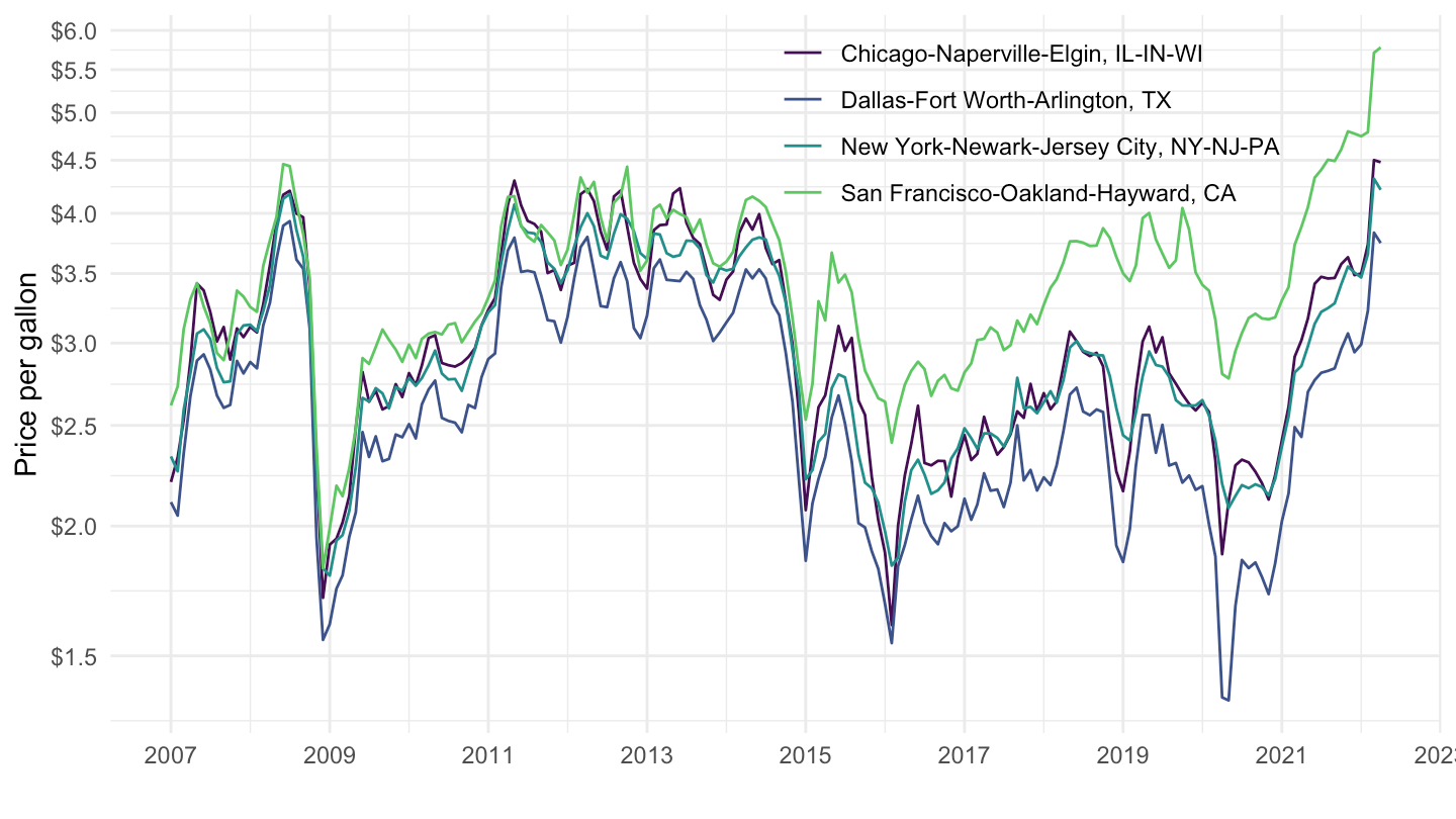

2012 -

ap.data |>
  left_join(ap.series, by = "series_id") |>
  left_join(ap.item, by = "item_code") |>
  left_join(ap.area, by = "area_code") |>
  filter(item_code %in% c("74714"),
         area_code %in% c("S49B", "S37A", "S23A", "S12A")) |>
  month_to_date() |>
  filter(date >= as.Date("2012-01-01")) |>
  ggplot() + theme_minimal() + xlab("") + ylab("Price per gallon") +
  geom_line(aes(x = date, y = value, color = area_name)) +
  scale_color_manual(values = viridis(5)[1:4]) +
  theme(legend.title = element_blank(),
        legend.position = c(0.45, 0.85)) +
  scale_y_log10(breaks = seq(0, 6, 0.5),
                labels = scales::dollar_format(accuracy = .1)) + 
  scale_x_date(breaks = as.Date(paste0(seq(1945, 2025, 1), "-01-01")),
               labels = date_format("%Y"))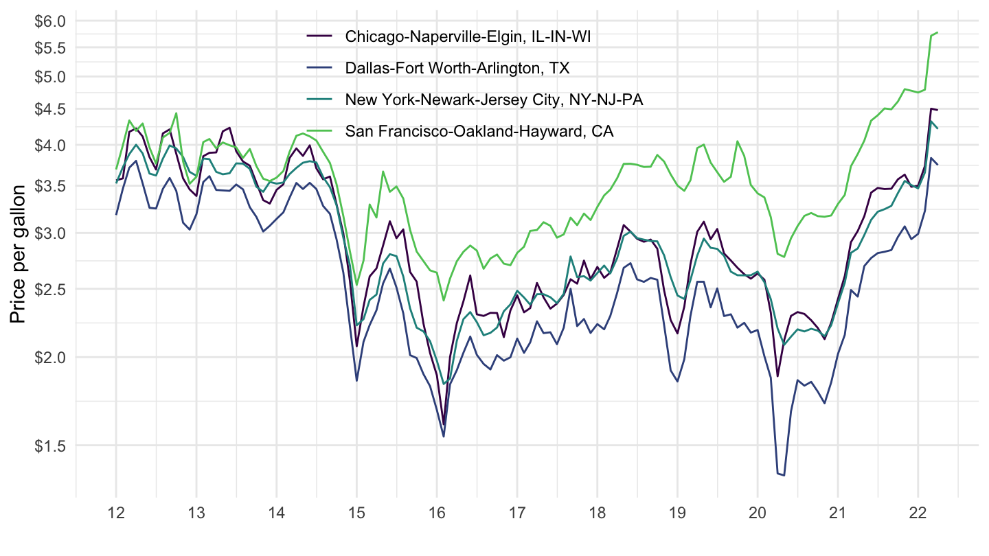

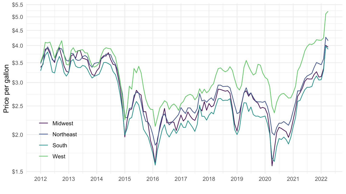
Midwest, Northeast, South, West

All

ap.data |>
  left_join(ap.series, by = "series_id") |>
  left_join(ap.item, by = "item_code") |>
  left_join(ap.area, by = "area_code") |>
  filter(item_code %in% c("74714"),
         area_code %in% c("0100", "0200", "0300", "0400")) |>
  month_to_date() |>
  ggplot() + theme_minimal() + xlab("") + ylab("Price per gallon") +
  geom_line(aes(x = date, y = value, color = area_name)) +
  scale_color_manual(values = viridis(5)[1:4]) +
  geom_rect(data = nber_recessions |>
              filter(Peak > as.Date("1976-01-01")), 
            aes(xmin = Peak, xmax = Trough, ymin = -Inf, ymax = +Inf), 
            fill = 'grey', alpha = 0.5) +
  theme(legend.title = element_blank(),
        legend.position = c(0.3, 0.8)) +
  scale_y_log10(breaks = seq(0, 6, 0.5),
                labels = scales::dollar_format(accuracy = .1)) + 
  scale_x_date(breaks = as.Date(paste0(seq(1945, 2025, 5), "-01-01")),
               labels = date_format("%Y"))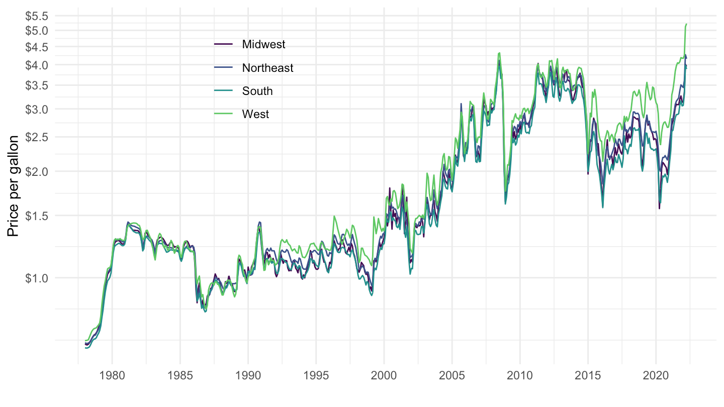

2007 -

ap.data |>
  left_join(ap.series, by = "series_id") |>
  left_join(ap.item, by = "item_code") |>
  left_join(ap.area, by = "area_code") |>
  filter(item_code %in% c("74714"),
         area_code %in% c("0100", "0200", "0300", "0400")) |>
  month_to_date() |>
  filter(date >= as.Date("2007-01-01")) |>
  ggplot() + theme_minimal() + xlab("") + ylab("Price per gallon") +
  geom_line(aes(x = date, y = value, color = area_name)) +
  scale_color_manual(values = viridis(5)[1:4]) +
  geom_rect(data = nber_recessions |>
              filter(Peak > as.Date("2007-01-01")), 
            aes(xmin = Peak, xmax = Trough, ymin = -Inf, ymax = +Inf), 
            fill = 'grey', alpha = 0.5) +
  theme(legend.title = element_blank(),
        legend.position = c(0.8, 0.85)) +
  scale_y_continuous(breaks = seq(0, 6, 0.5),
                labels = scales::dollar_format(accuracy = .1)) + 
  scale_x_date(breaks = as.Date(paste0(seq(1944, 2025, 2), "-01-01")),
               labels = date_format("%Y"))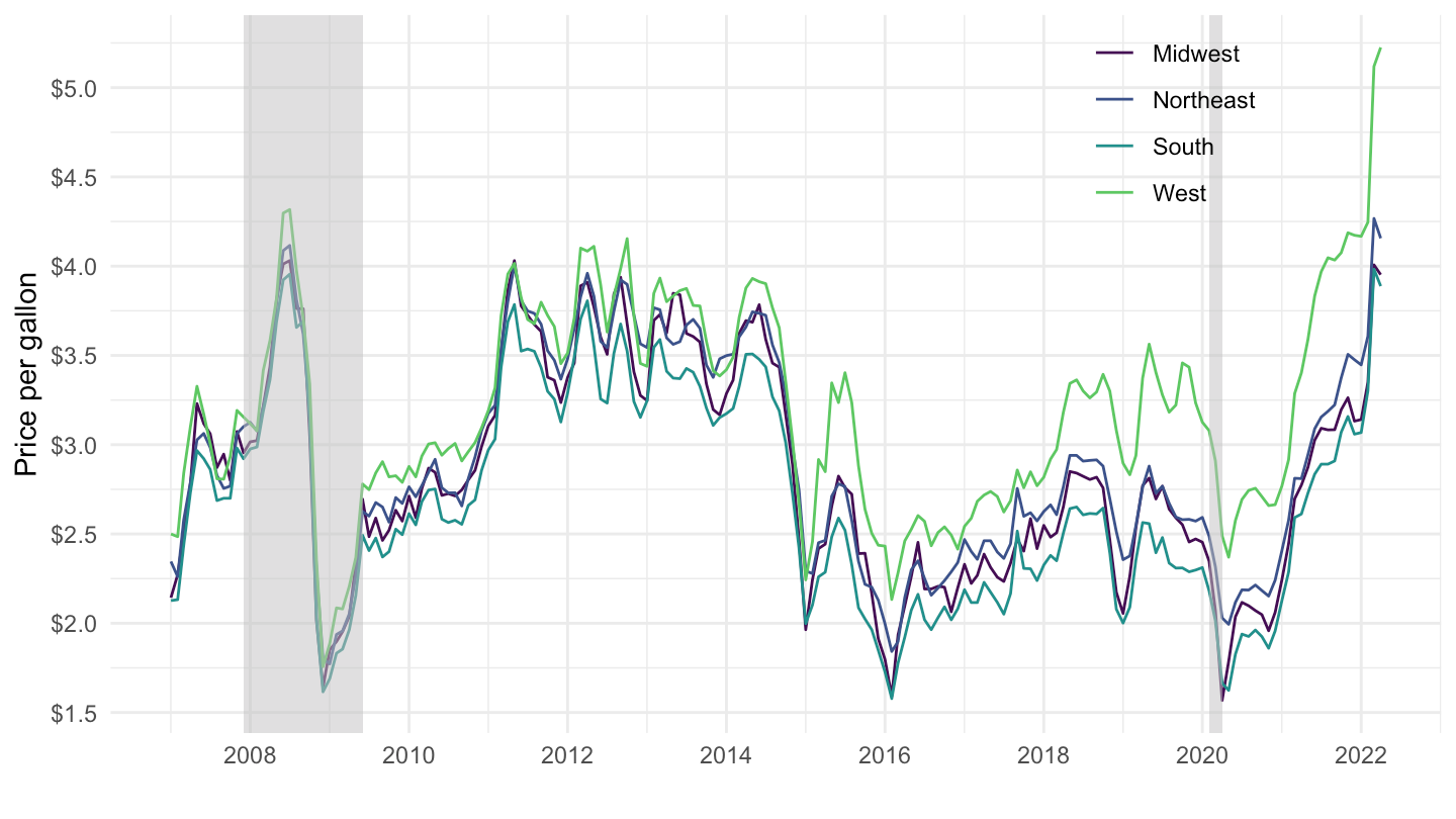

2012 -

ap.data |>
  left_join(ap.series, by = "series_id") |>
  left_join(ap.item, by = "item_code") |>
  left_join(ap.area, by = "area_code") |>
  filter(item_code %in% c("74714"),
         area_code %in% c("0100", "0200", "0300", "0400")) |>
  month_to_date() |>
  filter(date >= as.Date("2012-01-01")) |>
  ggplot() + theme_minimal() + xlab("") + ylab("Price per gallon") +
  geom_line(aes(x = date, y = value, color = area_name)) +
  scale_color_manual(values = viridis(5)[1:4]) +
  theme(legend.title = element_blank(),
        legend.position = c(0.1, 0.2)) +
  scale_y_log10(breaks = seq(0, 6, 0.5),
                labels = scales::dollar_format(accuracy = .1)) + 
  scale_x_date(breaks = as.Date(paste0(seq(1944, 2025, 1), "-01-01")),
               labels = date_format("%Y"))