BIS property prices - selected series - SPP

Data - BIS

Info

LAST_DOWNLOAD

LAST_DOWNLOAD
2022-05-27

LAST_COMPILE

LAST_COMPILE
2026-07-26

Last

SPP %>%
  group_by(date) %>%
  summarise(Nobs = n()) %>%
  arrange(desc(date)) %>%
  head(1) %>%
  print_table_conditional()

date	Nobs
2026-01-01	104

REF_AREA, Reference area

SPP %>%
  left_join(REF_AREA, by = "REF_AREA") %>%
  group_by(REF_AREA, `Reference area`) %>%
  summarise(Nobs = n()) %>%
  arrange(-Nobs) %>%
  mutate(Flag = gsub(" ", "-", str_to_lower(`Reference area`)),
         Flag = paste0('<img src="../../icon/flag/vsmall/', Flag, '.png" alt="Flag">')) %>%
  select(Flag, everything()) %>%
  {if (is_html_output()) datatable(., filter = 'top', rownames = F, escape = F) else .}

Real House Prices

Thailand, South Korea, Japan

All

SPP %>%
  filter(REF_AREA %in% c("JP", "KR", "TH"),
         FREQ == "Q",
         VALUE == "R",
         UNIT_MEASURE == "628") %>%
  left_join(REF_AREA, by = "REF_AREA") %>%
  left_join(colors, by = c("Reference area" = "country")) %>%
  ggplot(.) + theme_minimal() + xlab("") + ylab("Real House Prices (Index, 2010 = 100)") +
  geom_line(aes(x = date, y = value, color = color)) + 
  scale_color_identity() + add_flags +
  scale_x_date(breaks = seq(1900, 2100, 5) %>% paste0("-01-01") %>% as.Date,
               labels = date_format("%Y")) +
  scale_y_log10(breaks = seq(0, 600, 10),
                     labels = dollar_format(a = 1, prefix = "")) +
  theme(legend.position = c(0.8, 0.2),
        legend.title = element_blank())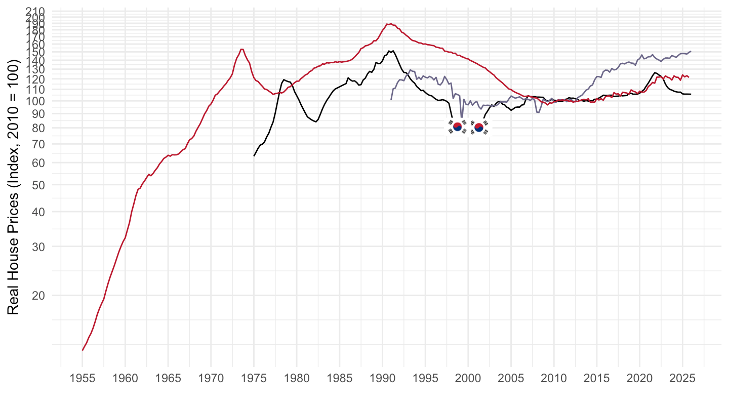

1975

SPP %>%
  filter(REF_AREA %in% c("JP", "KR", "TH"),
         FREQ == "Q",
         date >= as.Date("1980-01-01"),
         VALUE == "R",
         UNIT_MEASURE == "628") %>%
  left_join(REF_AREA, by = "REF_AREA") %>%
  left_join(colors, by = c("Reference area" = "country")) %>%
  ggplot(.) + theme_minimal() + xlab("") + ylab("Real House Prices (Index, 2010 = 100)") +
  geom_line(aes(x = date, y = value, color = color)) + 
  scale_color_identity() + add_flags +
  scale_x_date(breaks = seq(1900, 2100, 5) %>% paste0("-01-01") %>% as.Date,
               labels = date_format("%Y")) +
  scale_y_log10(breaks = seq(0, 600, 10),
                     labels = dollar_format(a = 1, prefix = "")) +
  theme(legend.position = c(0.8, 0.2),
        legend.title = element_blank())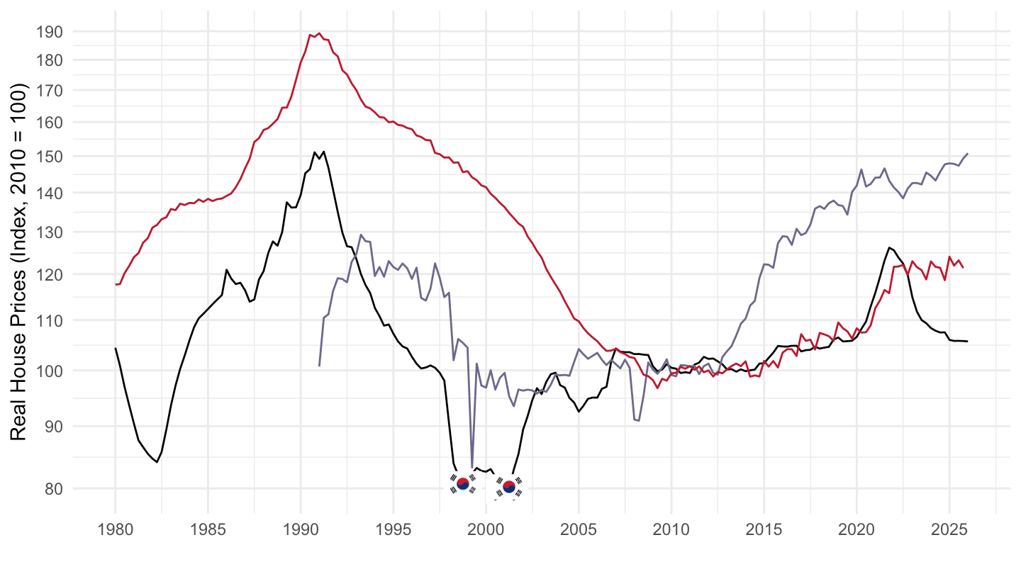

Japan, United States, United Kingdom

SPP %>%
  filter(REF_AREA %in% c("JP", "GB", "US"),
         FREQ == "Q",
         date >= as.Date("1970-01-01"),
         VALUE == "R",
         UNIT_MEASURE == "628") %>%
  left_join(REF_AREA, by = "REF_AREA") %>%
  left_join(colors, by = c("Reference area" = "country")) %>%
  ggplot(.) + theme_minimal() + xlab("") + ylab("Real House Prices (Index, 2010 = 100)") +
  geom_line(aes(x = date, y = value, color = color)) + 
  scale_color_identity() + add_flags +
  scale_x_date(breaks = seq(1900, 2100, 5) %>% paste0("-01-01") %>% as.Date,
               labels = date_format("%Y")) +
  scale_y_log10(breaks = seq(0, 600, 10),
                     labels = dollar_format(a = 1, prefix = "")) +
  theme(legend.position = c(0.8, 0.2),
        legend.title = element_blank())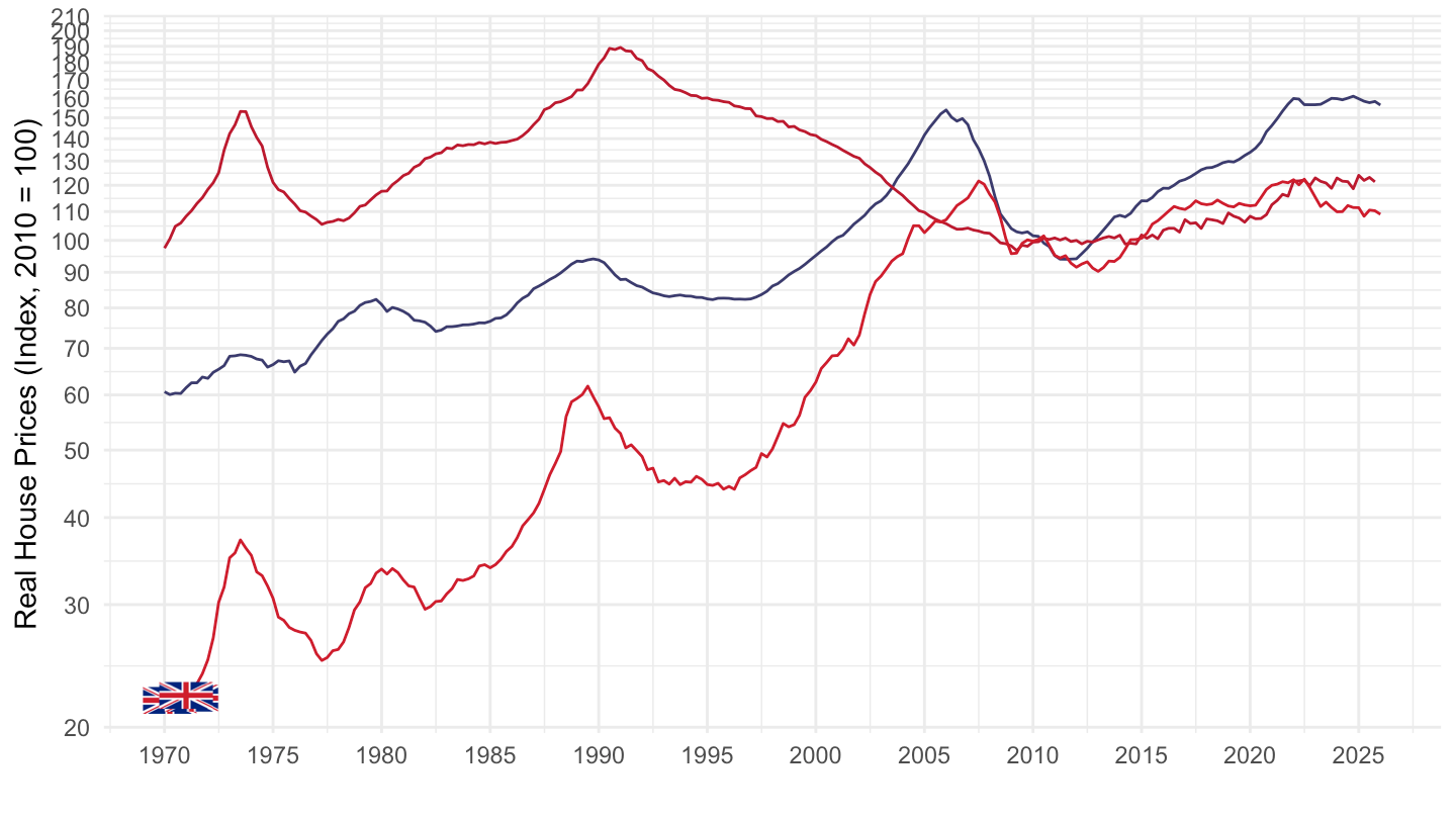

Germany, France, Italy

All

SPP %>%
  filter(REF_AREA %in% c("DE", "FR", "IT"),
         FREQ == "Q",
         date >= as.Date("1970-01-01"),
         VALUE == "R",
         UNIT_MEASURE == "628") %>%
  left_join(REF_AREA, by = "REF_AREA") %>%
  left_join(colors, by = c("Reference area" = "country")) %>%
  ggplot(.) + theme_minimal() + xlab("") + ylab("Real House Prices (Index, 2010 = 100)") +
  geom_line(aes(x = date, y = value, color = color)) + 
  scale_color_identity() + add_flags +
  scale_x_date(breaks = seq(1900, 2100, 5) %>% paste0("-01-01") %>% as.Date,
               labels = date_format("%Y")) +
  scale_y_log10(breaks = seq(0, 600, 10),
                     labels = dollar_format(a = 1, prefix = "")) +
  theme(legend.position = c(0.8, 0.2),
        legend.title = element_blank())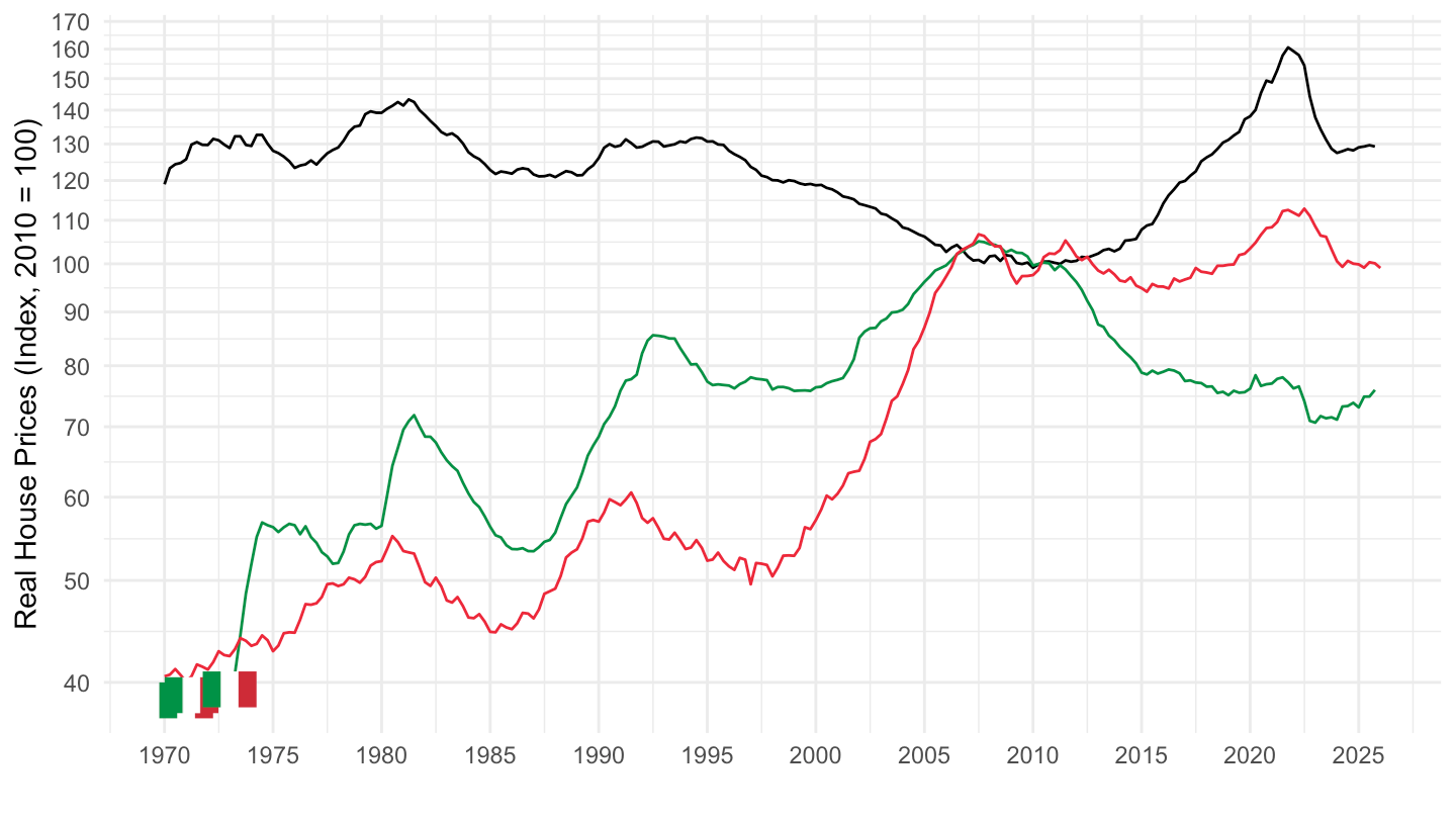

1998-

SPP %>%
  filter(REF_AREA %in% c("DEU", "FRA", "ITA"),
         FREQ == "Q",
         date >= as.Date("1997-12-31"),
         VALUE == "R",
         UNIT_MEASURE == 628) %>%
  left_join(colors, by = c("Reference area" = "country")) %>%
  group_by(REF_AREA) %>%
  mutate(value = 100*value/value[date == as.Date("1997-12-31")]) %>%
  ggplot(.) + theme_minimal() + xlab("") + ylab("Real House Prices (Index, 1998 = 100)") +
  geom_line(aes(x = date, y = value, color = color)) + 
  scale_color_identity() + add_flags +
  scale_x_date(breaks = seq(1900, 2100, 2) %>% paste0("-01-01") %>% as.Date,
               labels = date_format("%Y")) +
  scale_y_log10(breaks = seq(0, 600, 10),
                     labels = dollar_format(a = 1, prefix = "")) +
  theme(legend.position = c(0.8, 0.2),
        legend.title = element_blank())

2008-

SPP %>%
  filter(REF_AREA %in% c("DEU", "FRA", "ITA"),
         FREQ == "Q",
         date >= as.Date("2007-12-31"),
         VALUE == "R",
         UNIT_MEASURE == 628) %>%
  left_join(colors, by = c("Reference area" = "country")) %>%
  group_by(REF_AREA) %>%
  mutate(value = 100*value/value[date == as.Date("2007-12-31")]) %>%
  ggplot(.) + theme_minimal() + xlab("") + ylab("Real House Prices (Index, 1998 = 100)") +
  geom_line(aes(x = date, y = value, color = color)) + 
  scale_color_identity() + add_flags +
  scale_x_date(breaks = seq(1900, 2100, 2) %>% paste0("-01-01") %>% as.Date,
               labels = date_format("%Y")) +
  scale_y_log10(breaks = seq(0, 600, 10),
                     labels = dollar_format(a = 1, prefix = "")) +
  theme(legend.position = c(0.8, 0.2),
        legend.title = element_blank())

Germany, France, Italy, Japan, United States

All

SPP %>%
  filter(REF_AREA %in% c("DEU", "FRA", "ITA", "JPN", "USA"),
         FREQ == "Q",
         date >= as.Date("1970-01-01"),
         VALUE == "R",
         UNIT_MEASURE == 628) %>%
  left_join(colors, by = c("Reference area" = "country")) %>%
  mutate(color = ifelse(REF_AREA == "NLD", color2, color)) %>%
  ggplot(.) + theme_minimal() + xlab("") + ylab("Real House Prices (Index, 2010 = 100)") +
  geom_line(aes(x = date, y = value, color = color)) + 
  scale_color_identity() + add_flags +
  scale_x_date(breaks = seq(1900, 2100, 5) %>% paste0("-01-01") %>% as.Date,
               labels = date_format("%Y")) +
  scale_y_log10(breaks = seq(0, 600, 10),
                     labels = dollar_format(a = 1, prefix = "")) +
  theme(legend.position = c(0.8, 0.2),
        legend.title = element_blank())

1990-

SPP %>%
  filter(REF_AREA %in% c("DEU", "FRA", "ITA", "JPN", "USA", "ESP"),
         FREQ == "Q",
         date >= as.Date("1990-01-01"),
         VALUE == "R",
         UNIT_MEASURE == 628) %>%
  left_join(colors, by = c("Reference area" = "country")) %>%
  mutate(color = ifelse(REF_AREA == "NLD", color2, color)) %>%
  group_by(`Reference area`) %>%
  arrange(date) %>%
  mutate(value = 100*value/value[1]) %>%
  ggplot(.) + theme_minimal() + xlab("") + ylab("Real House Prices (Index, 2010 = 100)") +
  geom_line(aes(x = date, y = value, color = color)) + 
  scale_color_identity() + add_flags +
  scale_x_date(breaks = seq(1900, 2100, 5) %>% paste0("-01-01") %>% as.Date,
               labels = date_format("%Y")) +
  scale_y_log10(breaks = seq(0, 600, 10),
                     labels = dollar_format(a = 1, prefix = "")) +
  theme(legend.position = c(0.8, 0.2),
        legend.title = element_blank())

Germany, France, Italy, Spain, Netherlands

SPP %>%
  filter(REF_AREA %in% c("DEU", "FRA", "ITA", "ESP", "NLD"),
         FREQ == "Q",
         date >= as.Date("1970-01-01"),
         VALUE == "R",
         UNIT_MEASURE == 628) %>%
  left_join(colors, by = c("Reference area" = "country")) %>%
  mutate(color = ifelse(REF_AREA == "NLD", color2, color)) %>%
  ggplot(.) + theme_minimal() + xlab("") + ylab("Real House Prices (Index, 2010 = 100)") +
  geom_line(aes(x = date, y = value, color = color)) + 
  scale_color_identity() + add_flags +
  scale_x_date(breaks = seq(1900, 2100, 5) %>% paste0("-01-01") %>% as.Date,
               labels = date_format("%Y")) +
  scale_y_log10(breaks = seq(0, 600, 10),
                     labels = dollar_format(a = 1, prefix = "")) +
  theme(legend.position = c(0.8, 0.2),
        legend.title = element_blank())

Germany, France, Sweden, Japan

All

SPP %>%
  filter(REF_AREA %in% c("DEU", "FRA", "SWE", "JPN"),
         FREQ == "Q",
         date >= as.Date("1970-01-01"),
         VALUE == "R",
         UNIT_MEASURE == 628) %>%
  left_join(colors, by = c("Reference area" = "country")) %>%
  ggplot(.) + theme_minimal() + xlab("") + ylab("Real House Prices (Index, 2010 = 100)") +
  geom_line(aes(x = date, y = value, color = color)) + 
  scale_color_identity() + add_flags +
  scale_x_date(breaks = seq(1900, 2100, 5) %>% paste0("-01-01") %>% as.Date,
               labels = date_format("%Y")) +
  scale_y_log10(breaks = seq(0, 600, 10),
                     labels = dollar_format(a = 1, prefix = "")) +
  theme(legend.position = c(0.8, 0.2),
        legend.title = element_blank())

1998-

SPP %>%
  filter(REF_AREA %in% c("DEU", "FRA", "SWE", "JPN"),
         FREQ == "Q",
         date >= as.Date("1997-12-31"),
         VALUE == "R",
         UNIT_MEASURE == 628) %>%
  left_join(colors, by = c("Reference area" = "country")) %>%
  group_by(`Reference area`) %>%
  mutate(value = 100*value/value[date == as.Date("1997-12-31")]) %>%
  ggplot(.) + theme_minimal() + xlab("") + ylab("Real House Prices (Index, 1998 = 100)") +
  geom_line(aes(x = date, y = value, color = color)) + 
  scale_color_identity() + add_flags +
  scale_x_date(breaks = seq(1900, 2100, 2) %>% paste0("-01-01") %>% as.Date,
               labels = date_format("%Y")) +
  scale_y_log10(breaks = seq(0, 600, 10),
                     labels = dollar_format(a = 1, prefix = "")) +
  theme(legend.position = c(0.8, 0.2),
        legend.title = element_blank())

Germany, France, Sweden, Japan, Spain, US, Switzerland

All

SPP %>%
  filter(REF_AREA %in% c("DEU", "FRA", "SWE", "JPN", "ESP", "ITA", "USA", "CHE"),
         FREQ == "Q",
         VALUE == "R",
         date >= as.Date("1972-12-31"),
         UNIT_MEASURE == 628) %>%
  left_join(colors, by = c("Reference area" = "country")) %>%
  group_by(`Reference area`) %>%
  mutate(value = 100*value/value[date == as.Date("1972-12-31")]) %>%
  ggplot(.) + theme_minimal() + xlab("") + ylab("Real House Prices (Index, 1998 = 100)") +
  geom_line(aes(x = date, y = value, color = color)) + 
  scale_color_identity() + add_flags +
  scale_x_date(breaks = seq(1900, 2100, 5) %>% paste0("-01-01") %>% as.Date,
               labels = date_format("%Y")) +
  scale_y_log10(breaks = seq(0, 600, 10),
                     labels = dollar_format(a = 1, prefix = "")) +
  theme(legend.position = c(0.8, 0.2),
        legend.title = element_blank())

1998-

SPP %>%
  filter(REF_AREA %in% c("DEU", "FRA", "SWE", "JPN", "ESP", "ITA", "USA", "CHE"),
         FREQ == "Q",
         date >= as.Date("1997-12-31"),
         VALUE == "R",
         UNIT_MEASURE == 628) %>%
  left_join(colors, by = c("Reference area" = "country")) %>%
  group_by(`Reference area`) %>%
  mutate(value = 100*value/value[date == as.Date("1997-12-31")]) %>%
  ggplot(.) + theme_minimal() + xlab("") + ylab("Real House Prices (Index, 1998 = 100)") +
  geom_line(aes(x = date, y = value, color = color)) + 
  scale_color_identity() + add_flags +
  scale_x_date(breaks = seq(1900, 2100, 2) %>% paste0("-01-01") %>% as.Date,
               labels = date_format("%Y")) +
  scale_y_log10(breaks = seq(0, 600, 10),
                     labels = dollar_format(a = 1, prefix = "")) +
  theme(legend.position = c(0.8, 0.2),
        legend.title = element_blank())

Denmark, Germany, Switzerland

SPP %>%
  filter(REF_AREA %in% c("DEU", "DNK", "CHE"),
         FREQ == "Q",
         date >= as.Date("1970-01-01"),
         VALUE == "R",
         UNIT_MEASURE == 628) %>%
  left_join(colors, by = c("Reference area" = "country")) %>%
  ggplot(.) + theme_minimal() + xlab("") + ylab("Real House Prices (Index, 2010 = 100)") +
  geom_line(aes(x = date, y = value, color = color)) + 
  scale_color_identity() + add_flags +
  scale_x_date(breaks = seq(1900, 2100, 5) %>% paste0("-01-01") %>% as.Date,
               labels = date_format("%Y")) +
  scale_y_log10(breaks = seq(0, 600, 10),
                     labels = dollar_format(a = 1, prefix = "")) +
  theme(legend.position = c(0.8, 0.2),
        legend.title = element_blank())

Nominal House Prices

Japan, United States, United Kingdom

SPP %>%
  filter(REF_AREA %in% c("JPN", "GBR", "USA"),
         FREQ == "Q",
         date >= as.Date("1970-01-01"),
         VALUE == "N",
         UNIT_MEASURE == 628) %>%
  left_join(colors, by = c("Reference area" = "country")) %>%
  ggplot(.) + theme_minimal() + xlab("") + ylab("Real House Prices (Index, 2010 = 100)") +
  geom_line(aes(x = date, y = value, color = color)) + 
  scale_color_identity() + add_flags +
  scale_x_date(breaks = seq(1900, 2100, 5) %>% paste0("-01-01") %>% as.Date,
               labels = date_format("%Y")) +
  scale_y_log10(breaks = seq(0, 600, 10),
                     labels = dollar_format(a = 1, prefix = "")) +
  theme(legend.position = c(0.8, 0.2),
        legend.title = element_blank())

Germany, France, Sweden, Japan

1970-

SPP %>%
  filter(REF_AREA %in% c("DEU", "FRA", "JPN", "SWE"),
         FREQ == "Q",
         date >= as.Date("1970-01-01"),
         VALUE == "N",
         UNIT_MEASURE == 628) %>%
  left_join(colors, by = c("Reference area" = "country")) %>%
  ggplot(.) + theme_minimal() + xlab("") + ylab("Real House Prices (Index, 2010 = 100)") +
  geom_line(aes(x = date, y = value, color = color)) + 
  scale_color_identity() + add_flags +
  scale_x_date(breaks = seq(1900, 2100, 5) %>% paste0("-01-01") %>% as.Date,
               labels = date_format("%Y")) +
  scale_y_log10(breaks = seq(0, 600, 10),
                     labels = dollar_format(a = 1, prefix = "")) +
  theme(legend.position = c(0.8, 0.2),
        legend.title = element_blank())

1998-

SPP %>%
  filter(REF_AREA %in% c("DEU", "FRA", "JPN", "SWE"),
         FREQ == "Q",
         date >= as.Date("1998-01-01"),
         VALUE == "N",
         UNIT_MEASURE == 628) %>%
  left_join(colors, by = c("Reference area" = "country")) %>%
  ggplot(.) + theme_minimal() + xlab("") + ylab("Nominal House Prices (Index, 2010 = 100)") +
  geom_line(aes(x = date, y = value, color = color)) + 
  scale_color_identity() + add_flags +
  scale_x_date(breaks = seq(1900, 2100, 2) %>% paste0("-01-01") %>% as.Date,
               labels = date_format("%Y")) +
  scale_y_log10(breaks = seq(0, 600, 10),
                     labels = dollar_format(a = 1, prefix = "")) +
  theme(legend.position = c(0.8, 0.2),
        legend.title = element_blank())

Germany, France, Italy

SPP %>%
  filter(REF_AREA %in% c("DEU", "FRA", "ITA"),
         FREQ == "Q",
         date >= as.Date("1970-01-01"),
         VALUE == "N",
         UNIT_MEASURE == 628) %>%
  left_join(colors, by = c("Reference area" = "country")) %>%
  ggplot(.) + theme_minimal() + xlab("") + ylab("Real House Prices (Index, 2010 = 100)") +
  geom_line(aes(x = date, y = value, color = color)) + 
  scale_color_identity() + add_flags +
  scale_x_date(breaks = seq(1900, 2100, 5) %>% paste0("-01-01") %>% as.Date,
               labels = date_format("%Y")) +
  scale_y_log10(breaks = seq(0, 600, 10),
                     labels = dollar_format(a = 1, prefix = "")) +
  theme(legend.position = c(0.8, 0.2),
        legend.title = element_blank())

Denmark, Germany, Switzerland

SPP %>%
  filter(REF_AREA %in% c("DEU", "DNK", "CHE"),
         FREQ == "Q",
         date >= as.Date("1970-01-01"),
         VALUE == "N",
         UNIT_MEASURE == 628) %>%
  left_join(colors, by = c("Reference area" = "country")) %>%
  ggplot(.) + theme_minimal() + xlab("") + ylab("Real House Prices (Index, 2010 = 100)") +
  geom_line(aes(x = date, y = value, color = color)) + 
  scale_color_identity() + add_flags +
  scale_x_date(breaks = seq(1900, 2100, 5) %>% paste0("-01-01") %>% as.Date,
               labels = date_format("%Y")) +
  scale_y_log10(breaks = seq(0, 600, 10),
                     labels = dollar_format(a = 1, prefix = "")) +
  theme(legend.position = c(0.8, 0.2),
        legend.title = element_blank())

Individual Countries

Italy

SPP %>%
  filter(REF_AREA %in% c("ITA"),
         FREQ == "Q",
         UNIT_MEASURE == 628) %>%
  ggplot(.) + theme_minimal() + xlab("") + ylab("House Prices (Index, 2010 = 100)") +
  geom_line(aes(x = date, y = value, color = VALUE)) + 
  scale_x_date(breaks = seq(1900, 2100, 5) %>% paste0("-01-01") %>% as.Date,
               labels = date_format("%Y")) +
  scale_y_log10(breaks = seq(0, 600, 10),
                     labels = dollar_format(a = 1, prefix = "")) +
  scale_color_manual(values = viridis(3)[1:2]) +
  theme(legend.position = c(0.8, 0.2),
        legend.title = element_blank())

Japan

SPP %>%
  filter(REF_AREA %in% c("JPN"),
         FREQ == "Q",
         UNIT_MEASURE == 628) %>%
  ggplot(.) + theme_minimal() + xlab("") + ylab("House Prices (Index, 2010 = 100)") +
  geom_line(aes(x = date, y = value, color = VALUE)) + 
  scale_x_date(breaks = seq(1900, 2100, 5) %>% paste0("-01-01") %>% as.Date,
               labels = date_format("%Y")) +
  scale_y_log10(breaks = seq(0, 600, 10),
                     labels = dollar_format(a = 1, prefix = "")) +
  scale_color_manual(values = viridis(3)[1:2]) +
  theme(legend.position = c(0.8, 0.2),
        legend.title = element_blank())

South Africa

SPP %>%
  filter(REF_AREA %in% c("ZAF"),
         FREQ == "Q",
         UNIT_MEASURE == 628) %>%
  ggplot(.) + theme_minimal() + xlab("") + ylab("House Prices (Index, 2010 = 100)") +
  geom_line(aes(x = date, y = value, color = VALUE)) + 
  scale_x_date(breaks = seq(1900, 2100, 5) %>% paste0("-01-01") %>% as.Date,
               labels = date_format("%Y")) +
  scale_y_log10(breaks = seq(0, 600, 10),
                     labels = dollar_format(a = 1, prefix = "")) +
  scale_color_manual(values = viridis(3)[1:2]) +
  theme(legend.position = c(0.8, 0.2),
        legend.title = element_blank())

United Kingdom

SPP %>%
  filter(REF_AREA %in% c("GBR"),
         FREQ == "Q",
         UNIT_MEASURE == 628) %>%
  ggplot(.) + theme_minimal() + xlab("") + ylab("House Prices (Index, 2010 = 100)") +
  geom_line(aes(x = date, y = value, color = VALUE)) + 
  scale_x_date(breaks = seq(1900, 2100, 5) %>% paste0("-01-01") %>% as.Date,
               labels = date_format("%Y")) +
  scale_y_log10(breaks = seq(0, 600, 10),
                     labels = dollar_format(a = 1, prefix = "")) +
  scale_color_manual(values = viridis(3)[1:2]) +
  theme(legend.position = c(0.8, 0.2),
        legend.title = element_blank())

Australia

All

SPP %>%
  filter(REF_AREA %in% c("AUS"),
         FREQ == "Q",
         UNIT_MEASURE == 628) %>%
  ggplot(.) + theme_minimal() + xlab("") + ylab("House Prices (Index, 2010 = 100)") +
  geom_line(aes(x = date, y = value, color = VALUE)) + 
  scale_x_date(breaks = seq(1900, 2100, 5) %>% paste0("-01-01") %>% as.Date,
               labels = date_format("%Y")) +
  scale_y_log10(breaks = seq(0, 600, 10),
                     labels = dollar_format(a = 1, prefix = "")) +
  scale_color_manual(values = viridis(3)[1:2]) +
  theme(legend.position = c(0.8, 0.2),
        legend.title = element_blank())

2000-

SPP %>%
  filter(REF_AREA %in% c("AUS"),
         FREQ == "Q",
         UNIT_MEASURE == 628,
         date >= as.Date("2000-01-01")) %>%
  ggplot(.) + theme_minimal() + xlab("") + ylab("House Prices (Index, 2010 = 100)") +
  geom_line(aes(x = date, y = value, color = VALUE)) + 
  scale_x_date(breaks = seq(1900, 2100, 2) %>% paste0("-01-01") %>% as.Date,
               labels = date_format("%Y")) +
  scale_y_log10(breaks = seq(0, 600, 10),
                     labels = dollar_format(a = 1, prefix = "")) +
  scale_color_manual(values = viridis(3)[1:2]) +
  theme(legend.position = c(0.8, 0.2),
        legend.title = element_blank())

2010-

SPP %>%
  filter(REF_AREA %in% c("AUS"),
         FREQ == "Q",
         UNIT_MEASURE == 628,
         date >= as.Date("2010-01-01")) %>%
  ggplot(.) + theme_minimal() + xlab("") + ylab("House Prices (Index, 2010 = 100)") +
  geom_line(aes(x = date, y = value, color = VALUE)) + 
  scale_x_date(breaks = seq(1900, 2100, 1) %>% paste0("-01-01") %>% as.Date,
               labels = date_format("%Y")) +
  scale_y_log10(breaks = seq(0, 600, 10),
                     labels = dollar_format(a = 1, prefix = "")) +
  scale_color_manual(values = viridis(3)[1:2]) +
  theme(legend.position = c(0.8, 0.2),
        legend.title = element_blank())

Belgium

SPP %>%
  filter(REF_AREA %in% c("BEL"),
         FREQ == "Q",
         UNIT_MEASURE == 628) %>%
  ggplot(.) + theme_minimal() + xlab("") + ylab("House Prices (Index, 2010 = 100)") +
  geom_line(aes(x = date, y = value, color = VALUE)) + 
  scale_x_date(breaks = seq(1900, 2100, 5) %>% paste0("-01-01") %>% as.Date,
               labels = date_format("%Y")) +
  scale_y_log10(breaks = seq(0, 600, 10),
                     labels = dollar_format(a = 1, prefix = "")) +
  scale_color_manual(values = viridis(3)[1:2]) +
  theme(legend.position = c(0.8, 0.2),
        legend.title = element_blank())

Canada

SPP %>%
  filter(REF_AREA %in% c("CAN"),
         FREQ == "Q",
         UNIT_MEASURE == 628) %>%
  ggplot(.) + theme_minimal() + xlab("") + ylab("House Prices (Index, 2010 = 100)") +
  geom_line(aes(x = date, y = value, color = VALUE)) + 
  scale_x_date(breaks = seq(1900, 2100, 5) %>% paste0("-01-01") %>% as.Date,
               labels = date_format("%Y")) +
  scale_y_log10(breaks = seq(0, 600, 10),
                     labels = dollar_format(a = 1, prefix = "")) +
  scale_color_manual(values = viridis(3)[1:2]) +
  theme(legend.position = c(0.8, 0.2),
        legend.title = element_blank())

Switzerland

SPP %>%
  filter(REF_AREA %in% c("CHE"),
         FREQ == "Q",
         UNIT_MEASURE == 628) %>%
  ggplot(.) + theme_minimal() + xlab("") + ylab("House Prices (Index, 2010 = 100)") +
  geom_line(aes(x = date, y = value, color = VALUE)) + 
  scale_x_date(breaks = seq(1900, 2100, 5) %>% paste0("-01-01") %>% as.Date,
               labels = date_format("%Y")) +
  scale_y_log10(breaks = seq(0, 600, 10),
                     labels = dollar_format(a = 1, prefix = "")) +
  scale_color_manual(values = viridis(3)[1:2]) +
  theme(legend.position = c(0.8, 0.2),
        legend.title = element_blank())

Germany

SPP %>%
  filter(REF_AREA %in% c("DEU"),
         FREQ == "Q",
         UNIT_MEASURE == 628) %>%
  ggplot(.) + theme_minimal() + xlab("") + ylab("House Prices (Index, 2010 = 100)") +
  geom_line(aes(x = date, y = value, color = VALUE)) + 
  scale_x_date(breaks = seq(1900, 2100, 5) %>% paste0("-01-01") %>% as.Date,
               labels = date_format("%Y")) +
  scale_y_log10(breaks = seq(0, 600, 10),
                     labels = dollar_format(a = 1, prefix = "")) +
  scale_color_manual(values = viridis(3)[1:2]) +
  theme(legend.position = c(0.8, 0.2),
        legend.title = element_blank())

Denmark

SPP %>%
  filter(REF_AREA %in% c("DNK"),
         FREQ == "Q",
         UNIT_MEASURE == 628) %>%
  ggplot(.) + theme_minimal() + xlab("") + ylab("House Prices (Index, 2010 = 100)") +
  geom_line(aes(x = date, y = value, color = VALUE)) + 
  scale_x_date(breaks = seq(1900, 2100, 5) %>% paste0("-01-01") %>% as.Date,
               labels = date_format("%Y")) +
  scale_y_log10(breaks = seq(0, 600, 10),
                     labels = dollar_format(a = 1, prefix = "")) +
  scale_color_manual(values = viridis(3)[1:2]) +
  theme(legend.position = c(0.8, 0.2),
        legend.title = element_blank())

Finland

SPP %>%
  filter(REF_AREA %in% c("FIN"),
         FREQ == "Q",
         UNIT_MEASURE == 628) %>%
  ggplot(.) + theme_minimal() + xlab("") + ylab("House Prices (Index, 2010 = 100)") +
  geom_line(aes(x = date, y = value, color = VALUE)) + 
  scale_x_date(breaks = seq(1900, 2100, 5) %>% paste0("-01-01") %>% as.Date,
               labels = date_format("%Y")) +
  scale_y_log10(breaks = seq(0, 600, 10),
                     labels = dollar_format(a = 1, prefix = "")) +
  scale_color_manual(values = viridis(3)[1:2]) +
  theme(legend.position = c(0.8, 0.2),
        legend.title = element_blank())

France

SPP %>%
  filter(REF_AREA %in% c("FRA"),
         FREQ == "Q",
         date >= as.Date("1970-01-01"),
         UNIT_MEASURE == 628) %>%
  ggplot(.) + theme_minimal() + xlab("") + ylab("House Prices (Index, 2010 = 100)") +
  geom_line(aes(x = date, y = value, color = VALUE)) + 
  scale_x_date(breaks = seq(1900, 2100, 5) %>% paste0("-01-01") %>% as.Date,
               labels = date_format("%Y")) +
  scale_y_log10(breaks = c(seq(1, 10, 1), seq(0, 600, 10)),
                     labels = dollar_format(a = 1, prefix = "")) +
  scale_color_manual(values = viridis(3)[1:2]) +
  theme(legend.position = c(0.8, 0.2),
        legend.title = element_blank())

Ireland

SPP %>%
  filter(REF_AREA %in% c("IRL"),
         FREQ == "Q",
         UNIT_MEASURE == 628) %>%
  ggplot(.) + theme_minimal() + xlab("") + ylab("House Prices (Index, 2010 = 100)") +
  geom_line(aes(x = date, y = value, color = VALUE)) + 
  scale_x_date(breaks = seq(1900, 2100, 5) %>% paste0("-01-01") %>% as.Date,
               labels = date_format("%Y")) +
  scale_y_log10(breaks = seq(0, 600, 10),
                     labels = dollar_format(a = 1, prefix = "")) +
  scale_color_manual(values = viridis(3)[1:2]) +
  theme(legend.position = c(0.8, 0.2),
        legend.title = element_blank())

Netherlands

SPP %>%
  filter(REF_AREA %in% c("NLD"),
         FREQ == "Q",
         UNIT_MEASURE == 628) %>%
  ggplot(.) + theme_minimal() + xlab("") + ylab("House Prices (Index, 2010 = 100)") +
  geom_line(aes(x = date, y = value, color = VALUE)) + 
  scale_x_date(breaks = seq(1900, 2100, 5) %>% paste0("-01-01") %>% as.Date,
               labels = date_format("%Y")) +
  scale_y_log10(breaks = seq(0, 600, 10),
                     labels = dollar_format(a = 1, prefix = "")) +
  scale_color_manual(values = viridis(3)[1:2]) +
  theme(legend.position = c(0.8, 0.2),
        legend.title = element_blank())

New Zealand

SPP %>%
  filter(REF_AREA %in% c("NZL"),
         FREQ == "Q",
         UNIT_MEASURE == 628) %>%
  ggplot(.) + theme_minimal() + xlab("") + ylab("House Prices (Index, 2010 = 100)") +
  geom_line(aes(x = date, y = value, color = VALUE)) + 
  scale_x_date(breaks = seq(1900, 2100, 5) %>% paste0("-01-01") %>% as.Date,
               labels = date_format("%Y")) +
  scale_y_log10(breaks = seq(0, 600, 10),
                     labels = dollar_format(a = 1, prefix = "")) +
  scale_color_manual(values = viridis(3)[1:2]) +
  theme(legend.position = c(0.8, 0.2),
        legend.title = element_blank())

Sweden

SPP %>%
  filter(REF_AREA %in% c("SWE"),
         FREQ == "Q",
         UNIT_MEASURE == 628) %>%
  ggplot(.) + theme_minimal() + xlab("") + ylab("House Prices (Index, 2010 = 100)") +
  geom_line(aes(x = date, y = value, color = VALUE)) + 
  scale_x_date(breaks = seq(1900, 2100, 5) %>% paste0("-01-01") %>% as.Date,
               labels = date_format("%Y")) +
  scale_y_log10(breaks = seq(0, 600, 10),
                     labels = dollar_format(a = 1, prefix = "")) +
  scale_color_manual(values = viridis(3)[1:2]) +
  theme(legend.position = c(0.8, 0.2),
        legend.title = element_blank())

Sweden (1980 - 2000)

SPP %>%
  filter(REF_AREA %in% c("SWE"),
         FREQ == "Q",
         UNIT_MEASURE == 628,
         date >= as.Date("1980-01-01"),
         date <= as.Date("2000-01-01")) %>%
  ggplot(.) + theme_minimal() + xlab("") + ylab("House Prices (Index, 2010 = 100)") +
  geom_line(aes(x = date, y = value, color = VALUE)) + 
  scale_x_date(breaks = seq(1900, 2100, 2) %>% paste0("-01-01") %>% as.Date,
               labels = date_format("%Y")) +
  scale_y_log10(breaks = seq(0, 600, 5),
                     labels = dollar_format(a = 1, prefix = "")) +
  scale_color_manual(values = viridis(3)[1:2]) +
  theme(legend.position = c(0.8, 0.2),
        legend.title = element_blank())

United States

SPP %>%
  filter(REF_AREA %in% c("USA"),
         FREQ == "Q",
         UNIT_MEASURE == 628) %>%
  ggplot(.) + theme_minimal() + xlab("") + ylab("House Prices (Index, 2010 = 100)") +
  geom_line(aes(x = date, y = value, color = VALUE)) + 
  scale_x_date(breaks = seq(1900, 2100, 5) %>% paste0("-01-01") %>% as.Date,
               labels = date_format("%Y")) +
  scale_y_log10(breaks = seq(0, 600, 10),
                     labels = dollar_format(a = 1, prefix = "")) +
  scale_color_manual(values = viridis(3)[1:2]) +
  theme(legend.position = c(0.8, 0.2),
        legend.title = element_blank())

Spain

SPP %>%
  filter(REF_AREA %in% c("ESP"),
         FREQ == "Q",
         date >= as.Date("1970-01-01"),
         UNIT_MEASURE == 628) %>%
  ggplot(.) + theme_minimal() + xlab("") + ylab("House Prices (Index, 2010 = 100)") +
  geom_line(aes(x = date, y = value, color = VALUE)) + 
  scale_x_date(breaks = seq(1900, 2100, 5) %>% paste0("-01-01") %>% as.Date,
               labels = date_format("%Y")) +
  scale_y_log10(breaks = c(seq(1, 10, 1), seq(0, 600, 10)),
                     labels = dollar_format(a = 1, prefix = "")) +
  scale_color_manual(values = viridis(3)[1:2]) +
  theme(legend.position = c(0.8, 0.2),
        legend.title = element_blank())

Korea

SPP %>%
  filter(REF_AREA %in% c("KOR"),
         FREQ == "Q",
         date >= as.Date("1970-01-01"),
         UNIT_MEASURE == 628) %>%
  ggplot(.) + theme_minimal() + xlab("") + ylab("House Prices (Index, 2010 = 100)") +
  geom_line(aes(x = date, y = value, color = VALUE)) + 
  scale_x_date(breaks = seq(1900, 2100, 5) %>% paste0("-01-01") %>% as.Date,
               labels = date_format("%Y")) +
  scale_y_log10(breaks = c(seq(1, 10, 1), seq(0, 600, 10)),
                     labels = dollar_format(a = 1, prefix = "")) +
  scale_color_manual(values = viridis(3)[1:2]) +
  theme(legend.position = c(0.8, 0.2),
        legend.title = element_blank())

Euro Area

SPP %>%
  filter(`Reference area` %in% c("Euro area"),
         FREQ == "Q",
         UNIT_MEASURE == 628) %>%
  ggplot(.) + theme_minimal() + xlab("") + ylab("House Prices (Index, 2010 = 100)") +
  geom_line(aes(x = date, y = value, color = VALUE)) + 
  scale_x_date(breaks = seq(1900, 2100, 5) %>% paste0("-01-01") %>% as.Date,
               labels = date_format("%Y")) +
  scale_y_log10(breaks = seq(0, 600, 10),
                     labels = dollar_format(a = 1, prefix = "")) +
  scale_color_manual(values = viridis(3)[1:2]) +
  theme(legend.position = c(0.8, 0.2),
        legend.title = element_blank())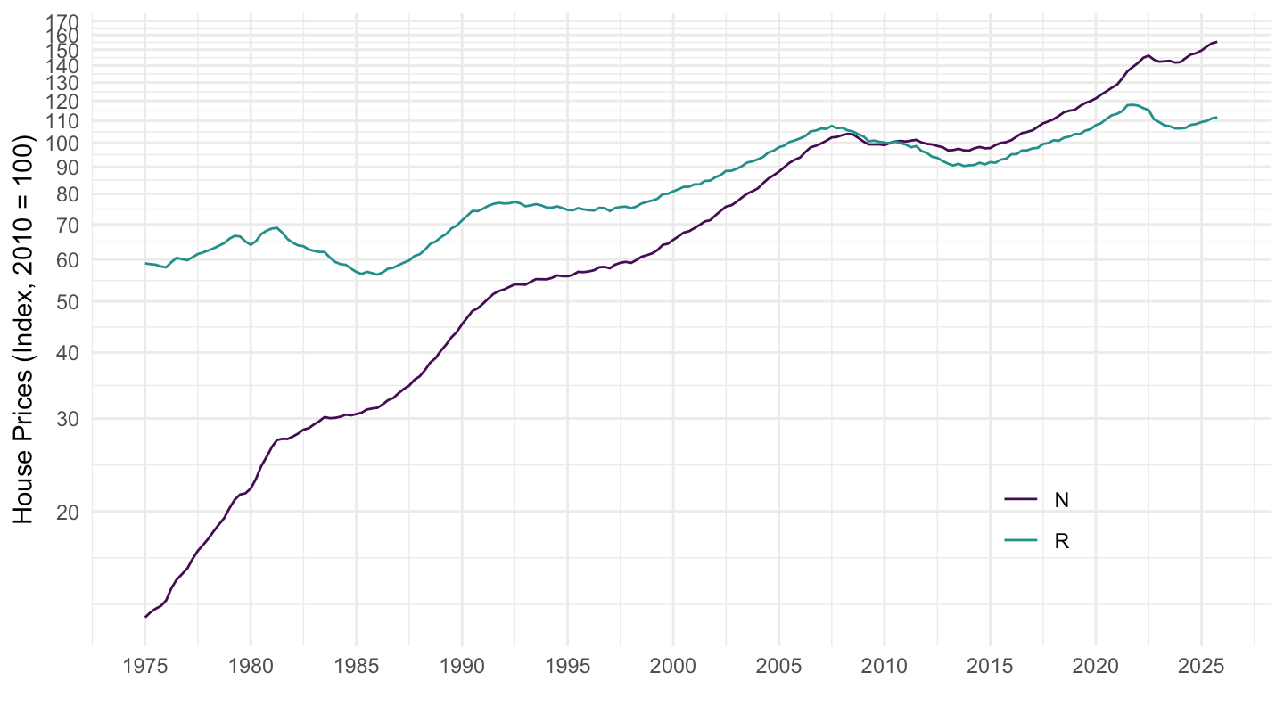

Hong Kong

SPP %>%
  filter(REF_AREA %in% c("HKG"),
         FREQ == "Q",
         UNIT_MEASURE == 628) %>%
  ggplot(.) + theme_minimal() + xlab("") + ylab("House Prices (Index, 2010 = 100)") +
  geom_line(aes(x = date, y = value, color = VALUE)) + 
  scale_x_date(breaks = seq(1900, 2100, 5) %>% paste0("-01-01") %>% as.Date,
               labels = date_format("%Y")) +
  scale_y_log10(breaks = seq(0, 600, 10),
                     labels = dollar_format(a = 1, prefix = "")) +
  scale_color_manual(values = viridis(3)[1:2]) +
  theme(legend.position = c(0.8, 0.2),
        legend.title = element_blank())

Norway

SPP %>%
  filter(REF_AREA %in% c("NOR"),
         FREQ == "Q",
         UNIT_MEASURE == 628) %>%
  ggplot(.) + theme_minimal() + xlab("") + ylab("House Prices (Index, 2010 = 100)") +
  geom_line(aes(x = date, y = value, color = VALUE)) + 
  scale_x_date(breaks = seq(1900, 2100, 5) %>% paste0("-01-01") %>% as.Date,
               labels = date_format("%Y")) +
  scale_y_log10(breaks = seq(0, 600, 10),
                     labels = dollar_format(a = 1, prefix = "")) +
  scale_color_manual(values = viridis(3)[1:2]) +
  theme(legend.position = c(0.8, 0.2),
        legend.title = element_blank())

Colombia

SPP %>%
  filter(REF_AREA %in% c("COL"),
         FREQ == "Q",
         UNIT_MEASURE == 628) %>%
  ggplot(.) + theme_minimal() + xlab("") + ylab("House Prices (Index, 2010 = 100)") +
  geom_line(aes(x = date, y = value, color = VALUE)) + 
  scale_x_date(breaks = seq(1900, 2100, 5) %>% paste0("-01-01") %>% as.Date,
               labels = date_format("%Y")) +
  scale_y_log10(breaks = seq(0, 600, 10),
                     labels = dollar_format(a = 1, prefix = "")) +
  scale_color_manual(values = viridis(3)[1:2]) +
  theme(legend.position = c(0.8, 0.2),
        legend.title = element_blank())

Malaysia

SPP %>%
  filter(REF_AREA %in% c("MYS"),
         FREQ == "Q",
         UNIT_MEASURE == 628) %>%
  ggplot(.) + theme_minimal() + xlab("") + ylab("House Prices (Index, 2010 = 100)") +
  geom_line(aes(x = date, y = value, color = VALUE)) + 
  scale_x_date(breaks = seq(1900, 2100, 5) %>% paste0("-01-01") %>% as.Date,
               labels = date_format("%Y")) +
  scale_y_log10(breaks = seq(0, 600, 10),
                     labels = dollar_format(a = 1, prefix = "")) +
  scale_color_manual(values = viridis(3)[1:2]) +
  theme(legend.position = c(0.8, 0.2),
        legend.title = element_blank())

Thailand

SPP %>%
  filter(REF_AREA %in% c("THA"),
         FREQ == "Q",
         UNIT_MEASURE == 628) %>%
  ggplot(.) + theme_minimal() + xlab("") + ylab("House Prices (Index, 2010 = 100)") +
  geom_line(aes(x = date, y = value, color = VALUE)) + 
  scale_x_date(breaks = seq(1900, 2100, 5) %>% paste0("-01-01") %>% as.Date,
               labels = date_format("%Y")) +
  scale_y_log10(breaks = seq(0, 600, 10),
                     labels = dollar_format(a = 1, prefix = "")) +
  scale_color_manual(values = viridis(3)[1:2]) +
  theme(legend.position = c(0.8, 0.2),
        legend.title = element_blank())

Israel

SPP %>%
  filter(REF_AREA %in% c("ISR"),
         FREQ == "Q",
         UNIT_MEASURE == 628) %>%
  ggplot(.) + theme_minimal() + xlab("") + ylab("House Prices (Index, 2010 = 100)") +
  geom_line(aes(x = date, y = value, color = VALUE)) + 
  scale_x_date(breaks = seq(1900, 2100, 5) %>% paste0("-01-01") %>% as.Date,
               labels = date_format("%Y")) +
  scale_y_log10(breaks = seq(0, 600, 10),
                     labels = dollar_format(a = 1, prefix = "")) +
  scale_color_manual(values = viridis(3)[1:2]) +
  theme(legend.position = c(0.8, 0.2),
        legend.title = element_blank())

Peru

SPP %>%
  filter(REF_AREA %in% c("PER"),
         FREQ == "Q",
         UNIT_MEASURE == 628) %>%
  ggplot(.) + theme_minimal() + xlab("") + ylab("House Prices (Index, 2010 = 100)") +
  geom_line(aes(x = date, y = value, color = VALUE)) + 
  scale_x_date(breaks = seq(1900, 2100, 5) %>% paste0("-01-01") %>% as.Date,
               labels = date_format("%Y")) +
  scale_y_log10(breaks = seq(0, 600, 10),
                     labels = dollar_format(a = 1, prefix = "")) +
  scale_color_manual(values = viridis(3)[1:2]) +
  theme(legend.position = c(0.8, 0.2),
        legend.title = element_blank())

Singapore

SPP %>%
  filter(REF_AREA %in% c("SGP"),
         FREQ == "Q",
         UNIT_MEASURE == 628) %>%
  ggplot(.) + theme_minimal() + xlab("") + ylab("House Prices (Index, 2010 = 100)") +
  geom_line(aes(x = date, y = value, color = VALUE)) + 
  scale_x_date(breaks = seq(1900, 2100, 5) %>% paste0("-01-01") %>% as.Date,
               labels = date_format("%Y")) +
  scale_y_log10(breaks = seq(0, 600, 10),
                     labels = dollar_format(a = 1, prefix = "")) +
  scale_color_manual(values = viridis(3)[1:2]) +
  theme(legend.position = c(0.8, 0.2),
        legend.title = element_blank())

Lithuania

SPP %>%
  filter(REF_AREA %in% c("LTU"),
         FREQ == "Q",
         UNIT_MEASURE == 628) %>%
  ggplot(.) + theme_minimal() + xlab("") + ylab("House Prices (Index, 2010 = 100)") +
  geom_line(aes(x = date, y = value, color = VALUE)) + 
  scale_x_date(breaks = seq(1900, 2100, 5) %>% paste0("-01-01") %>% as.Date,
               labels = date_format("%Y")) +
  scale_y_log10(breaks = seq(0, 600, 10),
                     labels = dollar_format(a = 1, prefix = "")) +
  scale_color_manual(values = viridis(3)[1:2]) +
  theme(legend.position = c(0.8, 0.2),
        legend.title = element_blank())

Austria

SPP %>%
  filter(REF_AREA %in% c("AUT"),
         FREQ == "Q",
         UNIT_MEASURE == 628) %>%
  ggplot(.) + theme_minimal() + xlab("") + ylab("House Prices (Index, 2010 = 100)") +
  geom_line(aes(x = date, y = value, color = VALUE)) + 
  scale_x_date(breaks = seq(1900, 2100, 5) %>% paste0("-01-01") %>% as.Date,
               labels = date_format("%Y")) +
  scale_y_log10(breaks = seq(0, 600, 10),
                     labels = dollar_format(a = 1, prefix = "")) +
  scale_color_manual(values = viridis(3)[1:2]) +
  theme(legend.position = c(0.8, 0.2),
        legend.title = element_blank())

Iceland

SPP %>%
  filter(REF_AREA %in% c("ISL"),
         FREQ == "Q",
         UNIT_MEASURE == 628) %>%
  ggplot(.) + theme_minimal() + xlab("") + ylab("House Prices (Index, 2010 = 100)") +
  geom_line(aes(x = date, y = value, color = VALUE)) + 
  scale_x_date(breaks = seq(1900, 2100, 2) %>% paste0("-01-01") %>% as.Date,
               labels = date_format("%Y")) +
  scale_y_log10(breaks = seq(0, 600, 10),
                     labels = dollar_format(a = 1, prefix = "")) +
  scale_color_manual(values = viridis(3)[1:2]) +
  theme(legend.position = c(0.8, 0.2),
        legend.title = element_blank())

North Macedonia

SPP %>%
  filter(REF_AREA %in% c("MKD"),
         FREQ == "Q",
         UNIT_MEASURE == 628) %>%
  ggplot(.) + theme_minimal() + xlab("") + ylab("House Prices (Index, 2010 = 100)") +
  geom_line(aes(x = date, y = value, color = VALUE)) + 
  scale_x_date(breaks = seq(1900, 2100, 5) %>% paste0("-01-01") %>% as.Date,
               labels = date_format("%Y")) +
  scale_y_log10(breaks = seq(0, 600, 10),
                     labels = dollar_format(a = 1, prefix = "")) +
  scale_color_manual(values = viridis(3)[1:2]) +
  theme(legend.position = c(0.8, 0.2),
        legend.title = element_blank())

Serbia

SPP %>%
  filter(REF_AREA %in% c("SRB"),
         FREQ == "Q",
         UNIT_MEASURE == 628) %>%
  ggplot(.) + theme_minimal() + xlab("") + ylab("House Prices (Index, 2010 = 100)") +
  geom_line(aes(x = date, y = value, color = VALUE)) + 
  scale_x_date(breaks = seq(1900, 2100, 2) %>% paste0("-01-01") %>% as.Date,
               labels = date_format("%Y")) +
  scale_y_log10(breaks = seq(0, 600, 10),
                     labels = dollar_format(a = 1, prefix = "")) +
  scale_color_manual(values = viridis(3)[1:2]) +
  theme(legend.position = c(0.8, 0.2),
        legend.title = element_blank())

Brazil

SPP %>%
  filter(REF_AREA %in% c("BRA"),
         FREQ == "Q",
         UNIT_MEASURE == 628) %>%
  ggplot(.) + theme_minimal() + xlab("") + ylab("House Prices (Index, 2010 = 100)") +
  geom_line(aes(x = date, y = value, color = VALUE)) + 
  scale_x_date(breaks = seq(1900, 2100, 2) %>% paste0("-01-01") %>% as.Date,
               labels = date_format("%Y")) +
  scale_y_log10(breaks = seq(0, 600, 10),
                     labels = dollar_format(a = 1, prefix = "")) +
  scale_color_manual(values = viridis(3)[1:2]) +
  theme(legend.position = c(0.8, 0.2),
        legend.title = element_blank())

Russia

SPP %>%
  filter(REF_AREA %in% c("RUS"),
         FREQ == "Q",
         UNIT_MEASURE == 628) %>%
  ggplot(.) + theme_minimal() + xlab("") + ylab("House Prices (Index, 2010 = 100)") +
  geom_line(aes(x = date, y = value, color = VALUE)) + 
  scale_x_date(breaks = seq(1900, 2100, 2) %>% paste0("-01-01") %>% as.Date,
               labels = date_format("%Y")) +
  scale_y_log10(breaks = seq(0, 600, 10),
                     labels = dollar_format(a = 1, prefix = "")) +
  scale_color_manual(values = viridis(3)[1:2]) +
  theme(legend.position = c(0.8, 0.2),
        legend.title = element_blank())

Croatia

SPP %>%
  filter(REF_AREA %in% c("HRV"),
         FREQ == "Q",
         UNIT_MEASURE == 628) %>%
  ggplot(.) + theme_minimal() + xlab("") + ylab("House Prices (Index, 2010 = 100)") +
  geom_line(aes(x = date, y = value, color = VALUE)) + 
  scale_x_date(breaks = seq(1900, 2100, 2) %>% paste0("-01-01") %>% as.Date,
               labels = date_format("%Y")) +
  scale_y_log10(breaks = seq(0, 600, 10),
                     labels = dollar_format(a = 1, prefix = "")) +
  scale_color_manual(values = viridis(3)[1:2]) +
  theme(legend.position = c(0.8, 0.2),
        legend.title = element_blank())

Indonesia

SPP %>%
  filter(REF_AREA %in% c("IDN"),
         FREQ == "Q",
         UNIT_MEASURE == 628) %>%
  ggplot(.) + theme_minimal() + xlab("") + ylab("House Prices (Index, 2010 = 100)") +
  geom_line(aes(x = date, y = value, color = VALUE)) + 
  scale_x_date(breaks = seq(1900, 2100, 2) %>% paste0("-01-01") %>% as.Date,
               labels = date_format("%Y")) +
  scale_y_log10(breaks = seq(0, 600, 10),
                     labels = dollar_format(a = 1, prefix = "")) +
  scale_color_manual(values = viridis(3)[1:2]) +
  theme(legend.position = c(0.8, 0.2),
        legend.title = element_blank())

Chile

SPP %>%
  filter(REF_AREA %in% c("CHL"),
         FREQ == "Q",
         UNIT_MEASURE == 628) %>%
  ggplot(.) + theme_minimal() + xlab("") + ylab("House Prices (Index, 2010 = 100)") +
  geom_line(aes(x = date, y = value, color = VALUE)) + 
  scale_x_date(breaks = seq(1900, 2100, 2) %>% paste0("-01-01") %>% as.Date,
               labels = date_format("%Y")) +
  scale_y_log10(breaks = seq(0, 600, 10),
                     labels = dollar_format(a = 1, prefix = "")) +
  scale_color_manual(values = viridis(3)[1:2]) +
  theme(legend.position = c(0.8, 0.2),
        legend.title = element_blank())

Cyprus

SPP %>%
  filter(REF_AREA %in% c("CYP"),
         FREQ == "Q",
         UNIT_MEASURE == 628) %>%
  ggplot(.) + theme_minimal() + xlab("") + ylab("House Prices (Index, 2010 = 100)") +
  geom_line(aes(x = date, y = value, color = VALUE)) + 
  scale_x_date(breaks = seq(1900, 2100, 2) %>% paste0("-01-01") %>% as.Date,
               labels = date_format("%Y")) +
  scale_y_log10(breaks = seq(0, 600, 10),
                     labels = dollar_format(a = 1, prefix = "")) +
  scale_color_manual(values = viridis(3)[1:2]) +
  theme(legend.position = c(0.8, 0.2),
        legend.title = element_blank())

United Arab Emirates

SPP %>%
  filter(REF_AREA %in% c("ARE"),
         FREQ == "Q",
         UNIT_MEASURE == 628) %>%
  ggplot(.) + theme_minimal() + xlab("") + ylab("House Prices (Index, 2010 = 100)") +
  geom_line(aes(x = date, y = value, color = VALUE)) + 
  scale_x_date(breaks = seq(1900, 2100, 2) %>% paste0("-01-01") %>% as.Date,
               labels = date_format("%Y")) +
  scale_y_log10(breaks = seq(0, 600, 10),
                     labels = dollar_format(a = 1, prefix = "")) +
  scale_color_manual(values = viridis(3)[1:2]) +
  theme(legend.position = c(0.8, 0.2),
        legend.title = element_blank())

Bulgaria

SPP %>%
  filter(REF_AREA %in% c("BGR"),
         FREQ == "Q",
         UNIT_MEASURE == 628) %>%
  ggplot(.) + theme_minimal() + xlab("") + ylab("House Prices (Index, 2010 = 100)") +
  geom_line(aes(x = date, y = value, color = VALUE)) + 
  scale_x_date(breaks = seq(1900, 2100, 2) %>% paste0("-01-01") %>% as.Date,
               labels = date_format("%Y")) +
  scale_y_log10(breaks = seq(0, 600, 10),
                     labels = dollar_format(a = 1, prefix = "")) +
  scale_color_manual(values = viridis(3)[1:2]) +
  theme(legend.position = c(0.8, 0.2),
        legend.title = element_blank())

Estonia

SPP %>%
  filter(REF_AREA %in% c("EST"),
         FREQ == "Q",
         UNIT_MEASURE == 628) %>%
  ggplot(.) + theme_minimal() + xlab("") + ylab("House Prices (Index, 2010 = 100)") +
  geom_line(aes(x = date, y = value, color = VALUE)) + 
  scale_x_date(breaks = seq(1900, 2100, 2) %>% paste0("-01-01") %>% as.Date,
               labels = date_format("%Y")) +
  scale_y_log10(breaks = seq(0, 600, 10),
                     labels = dollar_format(a = 1, prefix = "")) +
  scale_color_manual(values = viridis(3)[1:2]) +
  theme(legend.position = c(0.8, 0.2),
        legend.title = element_blank())

Mexico

SPP %>%
  filter(REF_AREA %in% c("MEX"),
         FREQ == "Q",
         UNIT_MEASURE == 628) %>%
  ggplot(.) + theme_minimal() + xlab("") + ylab("House Prices (Index, 2010 = 100)") +
  geom_line(aes(x = date, y = value, color = VALUE)) + 
  scale_x_date(breaks = seq(1900, 2100, 2) %>% paste0("-01-01") %>% as.Date,
               labels = date_format("%Y")) +
  scale_y_log10(breaks = seq(0, 600, 10),
                     labels = dollar_format(a = 1, prefix = "")) +
  scale_color_manual(values = viridis(3)[1:2]) +
  theme(legend.position = c(0.8, 0.2),
        legend.title = element_blank())

Malta

SPP %>%
  filter(REF_AREA %in% c("MLT"),
         FREQ == "Q",
         UNIT_MEASURE == 628) %>%
  ggplot(.) + theme_minimal() + xlab("") + ylab("House Prices (Index, 2010 = 100)") +
  geom_line(aes(x = date, y = value, color = VALUE)) + 
  scale_x_date(breaks = seq(1900, 2100, 2) %>% paste0("-01-01") %>% as.Date,
               labels = date_format("%Y")) +
  scale_y_log10(breaks = seq(0, 600, 10),
                     labels = dollar_format(a = 1, prefix = "")) +
  scale_color_manual(values = viridis(3)[1:2]) +
  theme(legend.position = c(0.8, 0.2),
        legend.title = element_blank())

China

SPP %>%
  filter(REF_AREA %in% c("CHN"),
         FREQ == "Q",
         UNIT_MEASURE == 628) %>%
  ggplot(.) + theme_minimal() + xlab("") + ylab("House Prices (Index, 2010 = 100)") +
  geom_line(aes(x = date, y = value, color = VALUE)) + 
  scale_x_date(breaks = seq(1900, 2100, 2) %>% paste0("-01-01") %>% as.Date,
               labels = date_format("%Y")) +
  scale_y_log10(breaks = seq(0, 600, 10),
                     labels = dollar_format(a = 1, prefix = "")) +
  scale_color_manual(values = viridis(3)[1:2]) +
  theme(legend.position = c(0.8, 0.2),
        legend.title = element_blank())

Greece

SPP %>%
  filter(REF_AREA %in% c("GRC"),
         FREQ == "Q",
         UNIT_MEASURE == 628) %>%
  ggplot(.) + theme_minimal() + xlab("") + ylab("House Prices (Index, 2010 = 100)") +
  geom_line(aes(x = date, y = value, color = VALUE)) + 
  scale_x_date(breaks = seq(1900, 2100, 2) %>% paste0("-01-01") %>% as.Date,
               labels = date_format("%Y")) +
  scale_y_log10(breaks = seq(0, 600, 10),
                     labels = dollar_format(a = 1, prefix = "")) +
  scale_color_manual(values = viridis(3)[1:2]) +
  theme(legend.position = c(0.8, 0.2),
        legend.title = element_blank())

Latvia

SPP %>%
  filter(REF_AREA %in% c("LVA"),
         FREQ == "Q",
         UNIT_MEASURE == 628) %>%
  ggplot(.) + theme_minimal() + xlab("") + ylab("House Prices (Index, 2010 = 100)") +
  geom_line(aes(x = date, y = value, color = VALUE)) + 
  scale_x_date(breaks = seq(1900, 2100, 2) %>% paste0("-01-01") %>% as.Date,
               labels = date_format("%Y")) +
  scale_y_log10(breaks = seq(0, 600, 10),
                     labels = dollar_format(a = 1, prefix = "")) +
  scale_color_manual(values = viridis(3)[1:2]) +
  theme(legend.position = c(0.8, 0.2),
        legend.title = element_blank())

Morocco

SPP %>%
  filter(REF_AREA %in% c("MAR"),
         FREQ == "Q",
         UNIT_MEASURE == 628) %>%
  ggplot(.) + theme_minimal() + xlab("") + ylab("House Prices (Index, 2010 = 100)") +
  geom_line(aes(x = date, y = value, color = VALUE)) + 
  scale_x_date(breaks = seq(1900, 2100, 2) %>% paste0("-01-01") %>% as.Date,
               labels = date_format("%Y")) +
  scale_y_log10(breaks = seq(0, 600, 10),
                     labels = dollar_format(a = 1, prefix = "")) +
  scale_color_manual(values = viridis(3)[1:2]) +
  theme(legend.position = c(0.8, 0.2),
        legend.title = element_blank())

Slovak Republic

SPP %>%
  filter(REF_AREA %in% c("SVK"),
         FREQ == "Q",
         UNIT_MEASURE == 628) %>%
  ggplot(.) + theme_minimal() + xlab("") + ylab("House Prices (Index, 2010 = 100)") +
  geom_line(aes(x = date, y = value, color = VALUE)) + 
  scale_x_date(breaks = seq(1900, 2100, 2) %>% paste0("-01-01") %>% as.Date,
               labels = date_format("%Y")) +
  scale_y_log10(breaks = seq(0, 600, 10),
                     labels = dollar_format(a = 1, prefix = "")) +
  scale_color_manual(values = viridis(3)[1:2]) +
  theme(legend.position = c(0.8, 0.2),
        legend.title = element_blank())

Hungary

SPP %>%
  filter(REF_AREA %in% c("HUN"),
         FREQ == "Q",
         UNIT_MEASURE == 628) %>%
  ggplot(.) + theme_minimal() + xlab("") + ylab("House Prices (Index, 2010 = 100)") +
  geom_line(aes(x = date, y = value, color = VALUE)) + 
  scale_x_date(breaks = seq(1900, 2100, 2) %>% paste0("-01-01") %>% as.Date,
               labels = date_format("%Y")) +
  scale_y_log10(breaks = seq(0, 600, 10),
                     labels = dollar_format(a = 1, prefix = "")) +
  scale_color_manual(values = viridis(3)[1:2]) +
  theme(legend.position = c(0.8, 0.2),
        legend.title = element_blank())

Slovenia

SPP %>%
  filter(REF_AREA %in% c("SVN"),
         FREQ == "Q",
         UNIT_MEASURE == 628) %>%
  ggplot(.) + theme_minimal() + xlab("") + ylab("House Prices (Index, 2010 = 100)") +
  geom_line(aes(x = date, y = value, color = VALUE)) + 
  scale_x_date(breaks = seq(1900, 2100, 2) %>% paste0("-01-01") %>% as.Date,
               labels = date_format("%Y")) +
  scale_y_log10(breaks = seq(0, 600, 10),
                     labels = dollar_format(a = 1, prefix = "")) +
  scale_color_manual(values = viridis(3)[1:2]) +
  theme(legend.position = c(0.8, 0.2),
        legend.title = element_blank())

Luxembourg

SPP %>%
  filter(REF_AREA %in% c("LUX"),
         FREQ == "Q",
         UNIT_MEASURE == 628) %>%
  ggplot(.) + theme_minimal() + xlab("") + ylab("House Prices (Index, 2010 = 100)") +
  geom_line(aes(x = date, y = value, color = VALUE)) + 
  scale_x_date(breaks = seq(1900, 2100, 2) %>% paste0("-01-01") %>% as.Date,
               labels = date_format("%Y")) +
  scale_y_log10(breaks = seq(0, 600, 10),
                     labels = dollar_format(a = 1, prefix = "")) +
  scale_color_manual(values = viridis(3)[1:2]) +
  theme(legend.position = c(0.8, 0.2),
        legend.title = element_blank())

Czech Republic

SPP %>%
  filter(REF_AREA %in% c("CZE"),
         FREQ == "Q",
         UNIT_MEASURE == 628) %>%
  ggplot(.) + theme_minimal() + xlab("") + ylab("House Prices (Index, 2010 = 100)") +
  geom_line(aes(x = date, y = value, color = VALUE)) + 
  scale_x_date(breaks = seq(1900, 2100, 2) %>% paste0("-01-01") %>% as.Date,
               labels = date_format("%Y")) +
  scale_y_log10(breaks = seq(0, 600, 10),
                     labels = dollar_format(a = 1, prefix = "")) +
  scale_color_manual(values = viridis(3)[1:2]) +
  theme(legend.position = c(0.8, 0.2),
        legend.title = element_blank())

Philippines

SPP %>%
  filter(REF_AREA %in% c("PHL"),
         FREQ == "Q",
         UNIT_MEASURE == 628) %>%
  ggplot(.) + theme_minimal() + xlab("") + ylab("House Prices (Index, 2010 = 100)") +
  geom_line(aes(x = date, y = value, color = VALUE)) + 
  scale_x_date(breaks = seq(1900, 2100, 2) %>% paste0("-01-01") %>% as.Date,
               labels = date_format("%Y")) +
  scale_y_log10(breaks = seq(0, 600, 10),
                     labels = dollar_format(a = 1, prefix = "")) +
  scale_color_manual(values = viridis(3)[1:2]) +
  theme(legend.position = c(0.8, 0.2),
        legend.title = element_blank())

Portugal

SPP %>%
  filter(REF_AREA %in% c("PRT"),
         FREQ == "Q",
         UNIT_MEASURE == 628) %>%
  ggplot(.) + theme_minimal() + xlab("") + ylab("House Prices (Index, 2010 = 100)") +
  geom_line(aes(x = date, y = value, color = VALUE)) + 
  scale_x_date(breaks = seq(1900, 2100, 2) %>% paste0("-01-01") %>% as.Date,
               labels = date_format("%Y")) +
  scale_y_log10(breaks = seq(0, 600, 10),
                     labels = dollar_format(a = 1, prefix = "")) +
  scale_color_manual(values = viridis(3)[1:2]) +
  theme(legend.position = c(0.8, 0.2),
        legend.title = element_blank())

India

SPP %>%
  filter(REF_AREA %in% c("IND"),
         FREQ == "Q",
         UNIT_MEASURE == 628) %>%
  ggplot(.) + theme_minimal() + xlab("") + ylab("House Prices (Index, 2010 = 100)") +
  geom_line(aes(x = date, y = value, color = VALUE)) + 
  scale_x_date(breaks = seq(1900, 2100, 2) %>% paste0("-01-01") %>% as.Date,
               labels = date_format("%Y")) +
  scale_y_log10(breaks = seq(0, 600, 10),
                     labels = dollar_format(a = 1, prefix = "")) +
  scale_color_manual(values = viridis(3)[1:2]) +
  theme(legend.position = c(0.8, 0.2),
        legend.title = element_blank())

Romania

SPP %>%
  filter(REF_AREA %in% c("ROU"),
         FREQ == "Q",
         UNIT_MEASURE == 628) %>%
  ggplot(.) + theme_minimal() + xlab("") + ylab("House Prices (Index, 2010 = 100)") +
  geom_line(aes(x = date, y = value, color = VALUE)) + 
  scale_x_date(breaks = seq(1900, 2100, 2) %>% paste0("-01-01") %>% as.Date,
               labels = date_format("%Y")) +
  scale_y_log10(breaks = seq(0, 600, 10),
                     labels = dollar_format(a = 1, prefix = "")) +
  scale_color_manual(values = viridis(3)[1:2]) +
  theme(legend.position = c(0.8, 0.2),
        legend.title = element_blank())

Poland

SPP %>%
  filter(REF_AREA %in% c("POL"),
         FREQ == "Q",
         UNIT_MEASURE == 628) %>%
  ggplot(.) + theme_minimal() + xlab("") + ylab("House Prices (Index, 2010 = 100)") +
  geom_line(aes(x = date, y = value, color = VALUE)) + 
  scale_x_date(breaks = seq(1900, 2100, 2) %>% paste0("-01-01") %>% as.Date,
               labels = date_format("%Y")) +
  scale_y_log10(breaks = seq(0, 600, 10),
                     labels = dollar_format(a = 1, prefix = "")) +
  scale_color_manual(values = viridis(3)[1:2]) +
  theme(legend.position = c(0.8, 0.2),
        legend.title = element_blank())

Turkey

SPP %>%
  filter(REF_AREA %in% c("TUR"),
         FREQ == "Q",
         UNIT_MEASURE == 628) %>%
  ggplot(.) + theme_minimal() + xlab("") + ylab("House Prices (Index, 2010 = 100)") +
  geom_line(aes(x = date, y = value, color = VALUE)) + 
  scale_x_date(breaks = seq(1900, 2100, 2) %>% paste0("-01-01") %>% as.Date,
               labels = date_format("%Y")) +
  scale_y_log10(breaks = seq(0, 600, 10),
                     labels = dollar_format(a = 1, prefix = "")) +
  scale_color_manual(values = viridis(3)[1:2]) +
  theme(legend.position = c(0.2, 0.8),
        legend.title = element_blank())