Last observation: Q2 2026 (N = 36) · 2025 (N = 36)
First observation: 1929 (N = 21) · Q1 1947 (N = 21)
Last data update: 15 oct. 2026, 22:21
Last compile: 15 oct. 2026, 22:26
T40100_A |>
  group_by(LineNumber, LineDescription) |>
  summarise(Nobs = n())
# # A tibble: 36 × 3
# # Groups: LineNumber [36]
# LineNumber LineDescription Nobs
# <dbl> <chr> <int>
# 1 1 Current receipts from the rest of the world 97
# 2 2 Exports of goods and services 97
# 3 3 Goods 97
# 4 4 Durable 97
# 5 5 Nondurable 97
# 6 6 Services 97
# 7 7 Income receipts 97
# 8 8 Wage and salary receipts 78
# 9 9 Income receipts on assets 78
# 10 10 Interest 78
# # ℹ 26 more rowsT40100_A |>
year_to_date() |>
filter(LineNumber %in% c(1, 16, 19)) |>
group_by(date) |>
filter(n() == 3) |>
transmute(date,
`Exports` = DataValue[LineNumber == 16]/DataValue[LineNumber == 1],
`Imports` = DataValue[LineNumber == 19]/DataValue[LineNumber == 1]) |>
gather(variable, value, -date) |>
ggplot() + theme_minimal() + xlab("") + ylab("Exports, Imports (% of GDP)") +
geom_line(aes(x = date, y = value, color = variable, linetype = variable)) +
scale_x_date(breaks = seq(1920, 2100, 5) |> paste0("-01-01") |> as.Date(),
labels = date_format("%Y")) +
scale_color_manual(values = viridis(3)[1:2]) +
theme(legend.title = element_blank(),
legend.position = c(0.2, 0.9)) +
scale_y_continuous(breaks = seq(-0.06, 0.4, 0.02),
labels = scales::percent_format(accuracy = 1))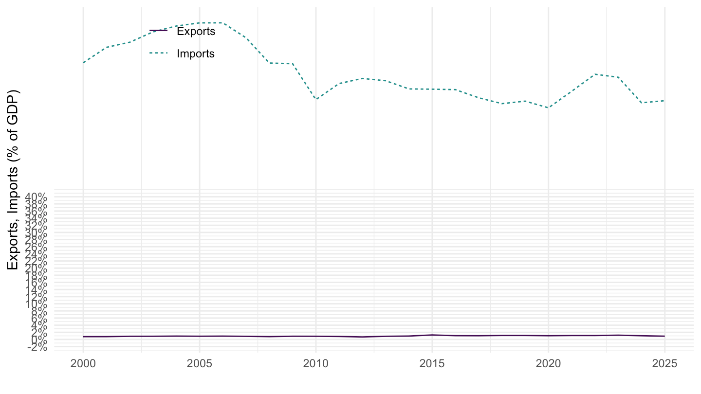
T40100_A |>
  year_to_date() |>
  filter(LineNumber %in% c(1, 17, 18, 20, 21)) |>
  group_by(date) |>
  filter(n() == 5) |>
  transmute(date,
            `Exports - Goods` = DataValue[LineNumber == 17]/DataValue[LineNumber == 1],
            `Exports - Services` = DataValue[LineNumber == 18]/DataValue[LineNumber == 1],
            `Imports - Goods` = DataValue[LineNumber == 20]/DataValue[LineNumber == 1],
            `Imports - Services` = DataValue[LineNumber == 21]/DataValue[LineNumber == 1]) |>
  gather(variable, value, -date) |>
  ggplot() + theme_minimal() + xlab("") +  ylab("Exports, Imports (% of GDP)") +
  geom_line(aes(x = date, y = value, color = variable, linetype = variable)) +
  scale_x_date(breaks = seq(1920, 2100, 5) |> paste0("-01-01") |> as.Date(),
               labels = date_format("%Y")) +
  scale_color_manual(values = c(viridis(3)[1], viridis(3)[2], viridis(3)[1], viridis(3)[2])) +
  scale_linetype_manual(values = c("dashed", "dashed", "solid",  "solid")) +
  theme(legend.title = element_blank(),
        legend.position = c(0.2, 0.9)) +
  scale_y_continuous(breaks = seq(-0.06, 0.4, 0.02),
                     labels = scales::percent_format(accuracy = 1))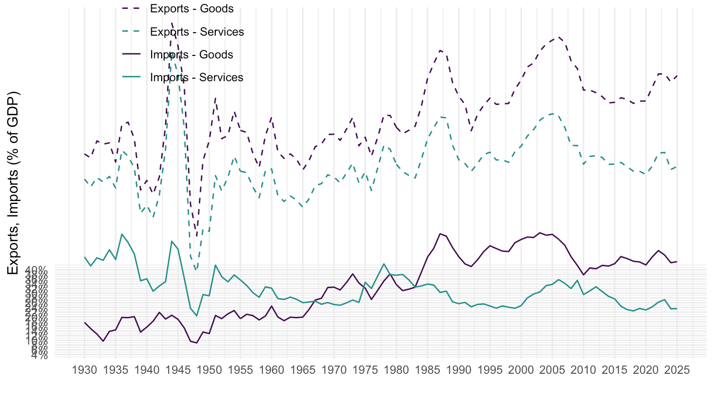
T40100_A |>
  year_to_date() |>
  filter(LineNumber %in% c(1, 17, 18, 20, 21)) |>
  group_by(date) |>
  filter(n() == 5) |>
  transmute(date,
            `Exports - Goods` = DataValue[LineNumber == 17]/DataValue[LineNumber == 1],
            `Exports - Services` = DataValue[LineNumber == 18]/DataValue[LineNumber == 1],
            `Imports - Goods` = DataValue[LineNumber == 20]/DataValue[LineNumber == 1],
            `Imports - Services` = DataValue[LineNumber == 21]/DataValue[LineNumber == 1]) |>
  gather(variable, value, -date) |>
  ggplot() + theme_minimal() + xlab("") +  ylab("Exports, Imports (% of GDP)") +
  geom_line(aes(x = date, y = value, color = variable, linetype = variable)) +
  scale_x_date(breaks = seq(1920, 2100, 5) |> paste0("-01-01") |> as.Date(),
               labels = date_format("%Y")) +
  scale_color_manual(values = c(viridis(3)[1], viridis(3)[2], viridis(3)[1], viridis(3)[2])) +
  scale_linetype_manual(values = c("dashed", "dashed", "solid",  "solid")) +
  geom_rect(data = nber_recessions |>
              filter(Peak > as.Date("1928-01-01")),
            aes(xmin = Peak, xmax = Trough, ymin = -Inf, ymax = +Inf),
            fill = 'grey', alpha = 0.5) +
  theme(legend.title = element_blank(),
        legend.position = c(0.2, 0.9)) +
  scale_y_continuous(breaks = seq(-0.06, 0.4, 0.02),
                     labels = scales::percent_format(accuracy = 1))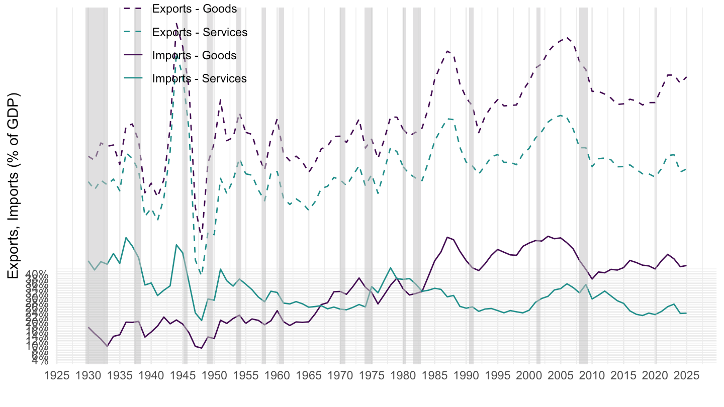
T40100_Q |>
  quarter_to_date() |>
  filter(LineNumber %in% c(1, 15)) |>
  group_by(date) |>
  filter(n() == 2) |>
  mutate(net_exports_gdp = DataValue[LineNumber == 15]/DataValue[LineNumber == 1]) |>
  ggplot() + theme_minimal() + xlab("") +  ylab("Net Exports (% of GDP)") +
  geom_line(aes(x = date, y = net_exports_gdp)) +
  scale_x_date(breaks = seq(1920, 2100, 5) |> paste0("-01-01") |> as.Date(),
               labels = date_format("%Y")) +
  theme(legend.title = element_blank(),
        legend.position = c(0.4, 0.8)) +
  scale_y_continuous(breaks = seq(-0.06, 0.05, 0.01),
                     labels = scales::percent_format(accuracy = 1)) +
  geom_hline(yintercept = 0, linetype = "dashed",  color = viridis(3)[2])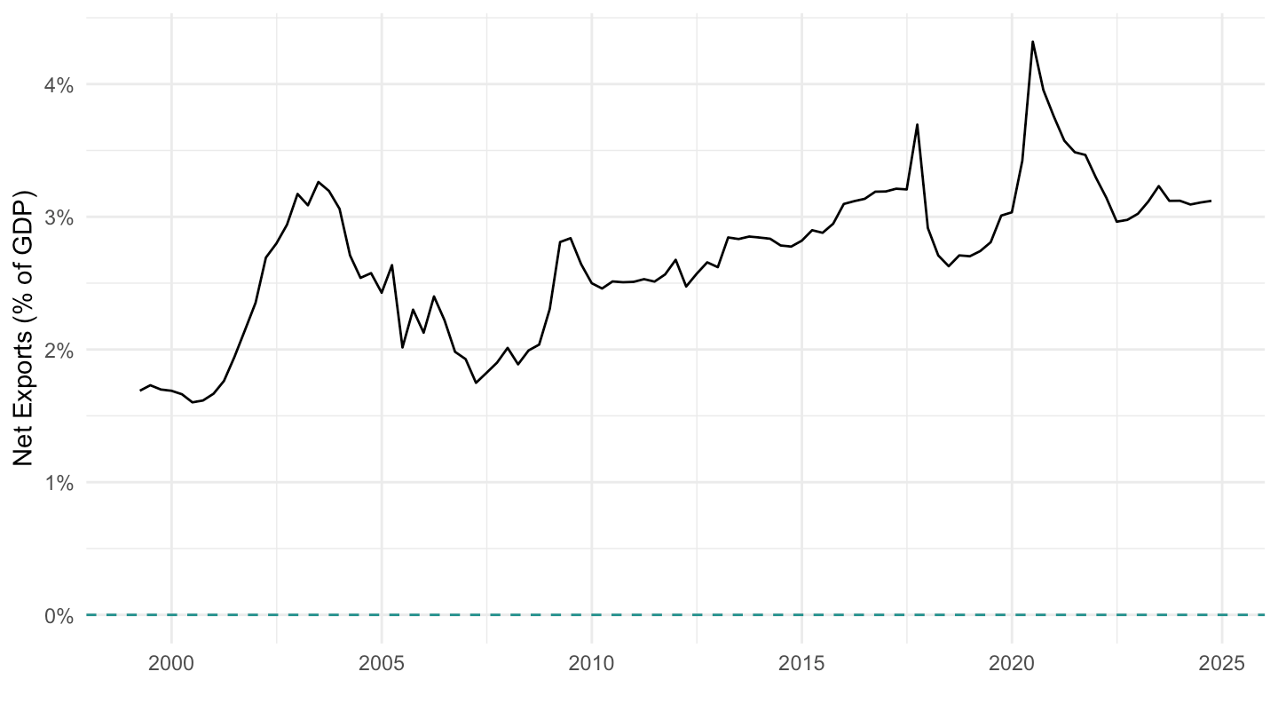
T40100_A |>
  year_to_date() |>
  filter(LineNumber %in% c(1, 15)) |>
  group_by(date) |>
  filter(n() == 2) |>
  mutate(net_exports_gdp = DataValue[LineNumber == 15]/DataValue[LineNumber == 1]) |>
  ggplot() + theme_minimal() + xlab("") +  ylab("Net Exports (% of GDP)") +
  geom_line(aes(x = date, y = net_exports_gdp)) +
  scale_x_date(breaks = seq(1920, 2100, 5) |> paste0("-01-01") |> as.Date(),
               labels = date_format("%Y")) +
  theme(legend.title = element_blank(),
        legend.position = c(0.4, 0.8)) +
  scale_y_continuous(breaks = seq(-0.06, 0.05, 0.01),
                     labels = scales::percent_format(accuracy = 1)) +
  geom_hline(yintercept = 0, linetype = "dashed",  color = viridis(3)[2])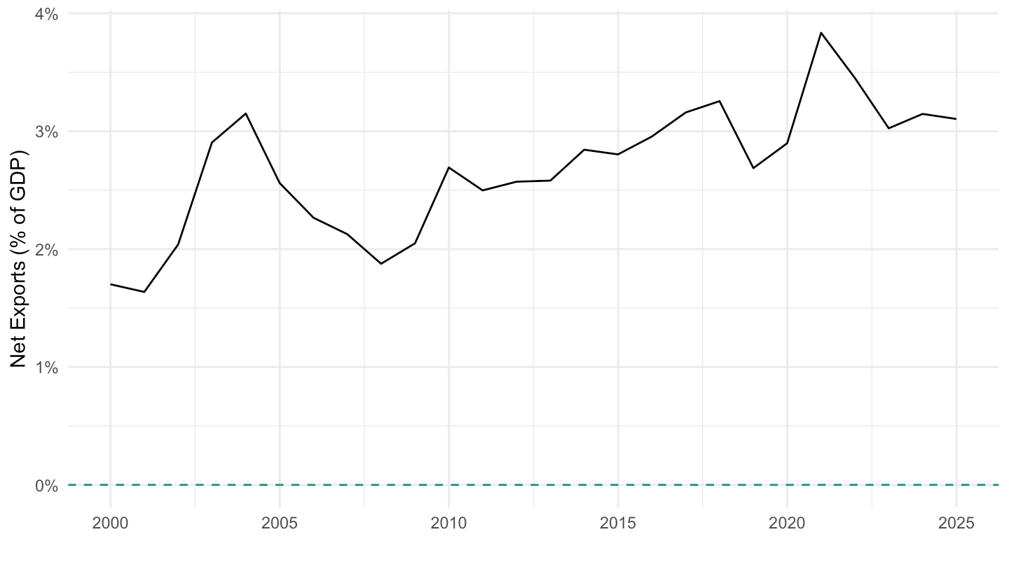
US_presidents_extract <- US_presidents |>
  filter(start >= as.Date("1945-01-01"))
T40100_Q |>
  quarter_to_date() |>
  filter(LineNumber %in% c(1, 15)) |>
  group_by(date) |>
  filter(n() == 2) |>
  mutate(net_exports_gdp = DataValue[LineNumber == 15]/DataValue[LineNumber == 1]) |>
  ggplot() + theme_minimal() + xlab("") +  ylab("Net Exports (% of GDP)") +
  geom_line(aes(x = date, y = net_exports_gdp)) +
  theme(legend.title = element_blank(),
        legend.position = c(0.4, 0.8)) +
  scale_x_date(breaks = as.Date(US_presidents_extract$start),
               labels = date_format("%Y")) +
  geom_vline(aes(xintercept = as.numeric(start)),
             data = US_presidents,
             colour = "grey50", alpha = 0.5) +
  geom_text(aes(x = start, y = new, label = name),
            data = US_presidents_extract |> mutate(new = -0.08 + 0.005 * (1:n() %% 2)),
            size = 2.5, vjust = 0, hjust = 0, nudge_x = 50) +
  geom_rect(aes(xmin = start, xmax = end, fill = party),
         ymin = -Inf, ymax = Inf, alpha = 0.1, data = US_presidents_extract) +
  scale_fill_manual(values = c("white", "grey")) +
  guides(color = guide_legend("party"), fill = FALSE) +
  scale_y_continuous(breaks = seq(-0.06, 0.05, 0.01),
                     labels = scales::percent_format(accuracy = 1)) +
  geom_hline(yintercept = 0, linetype = "dashed",  color = viridis(3)[2])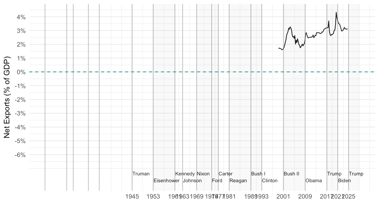
T40100_Q |>
  quarter_to_date() |>
  filter(LineNumber %in% c(1, 15),
         date >= as.Date("2016-12-01")) |>
  select(LineNumber, date, DataValue) |>
  spread(LineNumber, DataValue) %>%
{if (is_html_output()) datatable(., filter = 'top', rownames = F) else .}T40100_Q |>
quarter_to_date() |>
filter(LineNumber %in% c(1, 15),
date >= as.Date("2017-01-01")) |>
select(LineNumber, date, DataValue) |>
spread(LineNumber, DataValue) |>
ggplot() + geom_line(aes(x = date, y = `15`/1000)) +
theme_minimal() +
scale_x_date(breaks = as.Date(paste0(seq(1960, 2024, 1), "-01-01")),
labels = date_format("%Y")) +
theme(legend.position = c(0.2, 0.85),
legend.title = element_blank()) +
xlab("") + ylab("") +
scale_y_continuous(breaks = seq(-2000, 2000, 100),
labels = dollar_format(suffix = " Bn", accuracy = 1))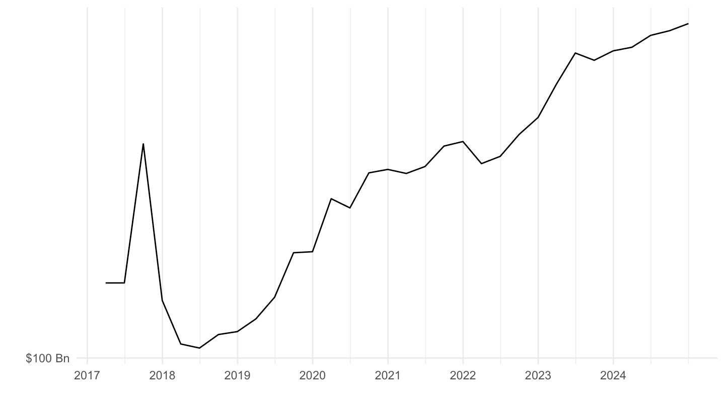
T40100_A |>
  year_to_date() |>
  mutate(year = year(date)) |>
  filter(year %in% c(1929, 1949, 1969, 1989, 2009, 2019)) |>
  group_by(year) |>
  mutate(value = round(100*DataValue/DataValue[1], 1)) |>
  ungroup() |>
  select(2, 3, 6, 7) |>
  spread(year, value) %>%
  mutate_at(vars(-1, -2), funs(ifelse(is.na(.), "", paste0(., " %")))) |>
  select(-LineNumber) %>%
  setNames(c("", names(.)[2:7])) |>
  knitr::kable(booktabs = TRUE,
               linesep = "") |>
  kable_styling(bootstrap_options = c("striped", "hover", "condensed"),
                latex_options = c("striped", "hold_position")) |>
  add_indent(c(2:26)) |>
  add_indent(c(3:6, 8:14, 16:21, 23:26)) |>
  add_indent(c(4:5, 9:13, 17:18, 20:21, 24:25)) |>
add_indent(c(10:12))| 1929 | 1949 | 1969 | 1989 | 2009 | 2019 | |
|---|---|---|---|---|---|---|
| Current receipts from the rest of the world | 100 % | 100 % | 100 % | 100 % | 100 % | 100 % |
| Exports of goods and services | 83.9 % | 88.2 % | 81.5 % | 73.9 % | 67 % | 65.5 % |
| Goods | 75.5 % | 74.3 % | 60.8 % | 54.9 % | 44.8 % | 42.4 % |
| Durable | 31.2 % | 37.1 % | 37.6 % | 35.6 % | 28.3 % | 25.4 % |
| Nondurable | 44.3 % | 37.3 % | 23.3 % | 19.4 % | 16.5 % | 17 % |
| Services | 8.4 % | 13.8 % | 20.7 % | 19 % | 22.2 % | 23.1 % |
| Income receipts | 16.1 % | 11.8 % | 18.5 % | 26.1 % | 29.2 % | 30.3 % |
| Wage and salary receipts | 0.7 % | 0.4 % | 0.1 % | 0.2 % | 0.2 % | |
| Income receipts on assets | 11.1 % | 18.1 % | 25.9 % | 28.9 % | 30.1 % | |
| Interest | 1.7 % | 5.5 % | 14.8 % | 7.9 % | 7.3 % | |
| Dividends | 6.8 % | 7.6 % | 7 % | 10 % | 18.2 % | |
| Reinvested earnings on U.S. direct investment abroad | 2.7 % | 5 % | 4.1 % | 11 % | 4.6 % | |
| Current taxes, contributions for government social insurance, and transfer receipts from the rest of the world | 3.8 % | 4.2 % | ||||
| To persons | 0.2 % | 0.2 % | ||||
| To business | 2.7 % | 2.9 % | ||||
| To government | 0.9 % | 1 % | ||||
| Current payments to the rest of the world | 89.1 % | 94.6 % | 97.5 % | 113.5 % | 116.2 % | 111.5 % |
| Imports of goods and services | 78.5 % | 56.3 % | 79.3 % | 86.7 % | 84.8 % | 80.4 % |
| Goods | 63 % | 41.8 % | 57.8 % | 71.1 % | 67.2 % | 64.9 % |
| Durable | 17.7 % | 12.9 % | 32.6 % | 45.5 % | 37.8 % | 42 % |
| Nondurable | 45.4 % | 28.9 % | 25.2 % | 25.6 % | 29.4 % | 22.9 % |
| Services | 15.4 % | 14.5 % | 21.5 % | 15.6 % | 17.5 % | 15.5 % |
| Income payments | 5.3 % | 4 % | 8.9 % | 22.4 % | 22.8 % | 23 % |
| Wage and salary payments | 0.3 % | 0.3 % | 0.3 % | 0.6 % | 0.5 % | |
| Income payments on assets | 3.7 % | 8.6 % | 22.1 % | 22.2 % | 22.5 % | |
| Interest | 1.1 % | 6.3 % | 20.9 % | 16 % | 13.5 % | |
| Dividends | 1.7 % | 1.6 % | 2.4 % | 5 % | 5.8 % | |
| Reinvested earnings on foreign direct investment in the United States | 0.9 % | 0.7 % | -1.2 % | 1.2 % | 3.2 % | |
| Current taxes and transfer payments to the rest of the world | 5.3 % | 34.3 % | 9.3 % | 4.5 % | 8.6 % | 8.1 % |
| From persons | 4.8 % | 3.1 % | 1.8 % | 1.7 % | 3 % | 2.6 % |
| From government | 0.5 % | 31.2 % | 7.1 % | 2.1 % | 2.7 % | 1.9 % |
| From business | 0 % | 0 % | 0.5 % | 0.7 % | 3 % | 3.5 % |
| Balance on current account, NIPAs | 10.9 % | 5.4 % | 2.5 % | -13.5 % | -16.2 % | -11.5 % |
| Net lending or net borrowing (-), NIPAs | 10.9 % | 5.4 % | 2.5 % | -13.6 % | -16.5 % | -11.7 % |
| Balance on current account, NIPAs | 10.9 % | 5.4 % | 2.5 % | -13.5 % | -16.2 % | -11.5 % |
| Less: Capital account transactions (net) | 0 % | 0.1 % | 0.3 % | 0.2 % |
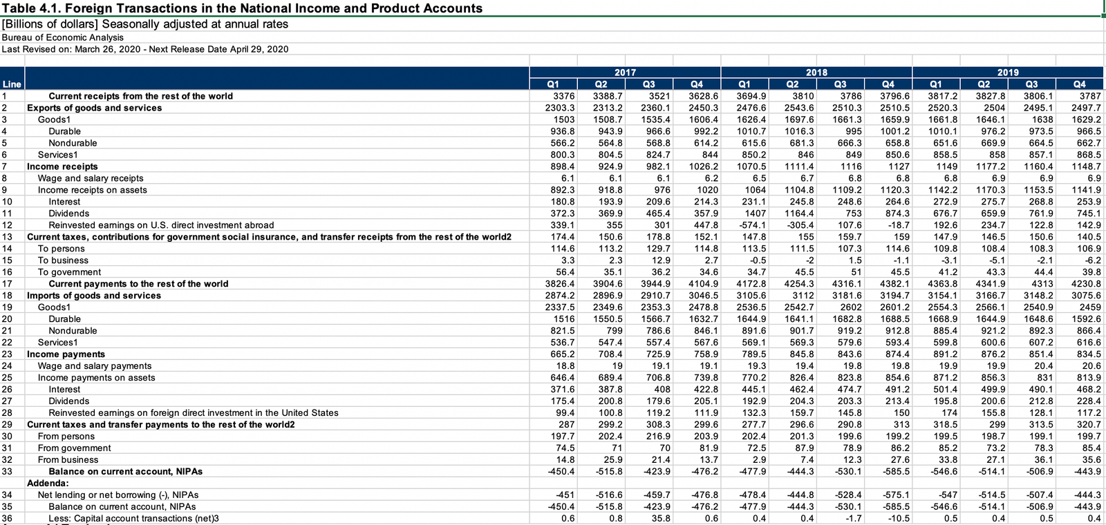
include_graphics2("https://fgeerolf.com/bib/bea/T40100_ex.png")
T40100_A |>
  year_to_date() |>
  mutate(year = year(date)) |>
  filter(year %in% c(1929, 1949, 1969, 1989, 2009, 2019)) |>
  group_by(year) |>
  mutate(value = round(DataValue/1000)) |>
  ungroup() |>
  select(2, 3, 6, 7) |>
  spread(year, value) %>%
  mutate_at(vars(-1, -2), funs(ifelse(is.na(.), "", paste0("$ ",., " Bn")))) |>
  select(-LineNumber) %>%
  setNames(c("", names(.)[2:7])) |>
  knitr::kable(booktabs = TRUE,
               linesep = "") |>
  kable_styling(bootstrap_options = c("striped", "hover", "condensed"),
                latex_options = c("striped", "hold_position")) |>
  add_indent(c(2:26)) |>
  add_indent(c(3:6, 8:14, 16:21, 23:26)) |>
  add_indent(c(4:5, 9:13, 17:18, 20:21, 24:25)) |>
add_indent(c(10:12))| 1929 | 1949 | 1969 | 1989 | 2009 | 2019 | |
|---|---|---|---|---|---|---|
| Current receipts from the rest of the world | $ 7 Bn | $ 16 Bn | $ 64 Bn | $ 682 Bn | $ 2362 Bn | $ 3876 Bn |
| Exports of goods and services | $ 6 Bn | $ 14 Bn | $ 52 Bn | $ 504 Bn | $ 1583 Bn | $ 2539 Bn |
| Goods | $ 5 Bn | $ 12 Bn | $ 39 Bn | $ 375 Bn | $ 1057 Bn | $ 1645 Bn |
| Durable | $ 2 Bn | $ 6 Bn | $ 24 Bn | $ 243 Bn | $ 668 Bn | $ 985 Bn |
| Nondurable | $ 3 Bn | $ 6 Bn | $ 15 Bn | $ 132 Bn | $ 390 Bn | $ 659 Bn |
| Services | $ 1 Bn | $ 2 Bn | $ 13 Bn | $ 130 Bn | $ 525 Bn | $ 895 Bn |
| Income receipts | $ 1 Bn | $ 2 Bn | $ 12 Bn | $ 178 Bn | $ 689 Bn | $ 1175 Bn |
| Wage and salary receipts | $ 0 Bn | $ 0 Bn | $ 1 Bn | $ 6 Bn | $ 7 Bn | |
| Income receipts on assets | $ 2 Bn | $ 12 Bn | $ 177 Bn | $ 684 Bn | $ 1168 Bn | |
| Interest | $ 0 Bn | $ 3 Bn | $ 101 Bn | $ 187 Bn | $ 284 Bn | |
| Dividends | $ 1 Bn | $ 5 Bn | $ 48 Bn | $ 237 Bn | $ 706 Bn | |
| Reinvested earnings on U.S. direct investment abroad | $ 0 Bn | $ 3 Bn | $ 28 Bn | $ 260 Bn | $ 178 Bn | |
| Current taxes, contributions for government social insurance, and transfer receipts from the rest of the world | $ 90 Bn | $ 162 Bn | ||||
| To persons | $ 6 Bn | $ 9 Bn | ||||
| To business | $ 64 Bn | $ 112 Bn | ||||
| To government | $ 21 Bn | $ 40 Bn | ||||
| Current payments to the rest of the world | $ 6 Bn | $ 16 Bn | $ 62 Bn | $ 774 Bn | $ 2745 Bn | $ 4323 Bn |
| Imports of goods and services | $ 6 Bn | $ 9 Bn | $ 50 Bn | $ 591 Bn | $ 2002 Bn | $ 3117 Bn |
| Goods | $ 4 Bn | $ 7 Bn | $ 37 Bn | $ 485 Bn | $ 1588 Bn | $ 2517 Bn |
| Durable | $ 1 Bn | $ 2 Bn | $ 21 Bn | $ 310 Bn | $ 893 Bn | $ 1628 Bn |
| Nondurable | $ 3 Bn | $ 5 Bn | $ 16 Bn | $ 175 Bn | $ 695 Bn | $ 888 Bn |
| Services | $ 1 Bn | $ 2 Bn | $ 14 Bn | $ 106 Bn | $ 414 Bn | $ 600 Bn |
| Income payments | $ 0 Bn | $ 1 Bn | $ 6 Bn | $ 153 Bn | $ 539 Bn | $ 893 Bn |
| Wage and salary payments | $ 0 Bn | $ 0 Bn | $ 2 Bn | $ 14 Bn | $ 19 Bn | |
| Income payments on assets | $ 1 Bn | $ 5 Bn | $ 151 Bn | $ 525 Bn | $ 874 Bn | |
| Interest | $ 0 Bn | $ 4 Bn | $ 142 Bn | $ 377 Bn | $ 523 Bn | |
| Dividends | $ 0 Bn | $ 1 Bn | $ 16 Bn | $ 119 Bn | $ 227 Bn | |
| Reinvested earnings on foreign direct investment in the United States | $ 0 Bn | $ 0 Bn | $ -8 Bn | $ 29 Bn | $ 124 Bn | |
| Current taxes and transfer payments to the rest of the world | $ 0 Bn | $ 6 Bn | $ 6 Bn | $ 30 Bn | $ 204 Bn | $ 314 Bn |
| From persons | $ 0 Bn | $ 1 Bn | $ 1 Bn | $ 12 Bn | $ 70 Bn | $ 102 Bn |
| From government | $ 0 Bn | $ 5 Bn | $ 5 Bn | $ 14 Bn | $ 63 Bn | $ 74 Bn |
| From business | $ 0 Bn | $ 0 Bn | $ 0 Bn | $ 5 Bn | $ 72 Bn | $ 137 Bn |
| Balance on current account, NIPAs | $ 1 Bn | $ 1 Bn | $ 2 Bn | $ -92 Bn | $ -383 Bn | $ -447 Bn |
| Net lending or net borrowing (-), NIPAs | $ 1 Bn | $ 1 Bn | $ 2 Bn | $ -93 Bn | $ -389 Bn | $ -454 Bn |
| Balance on current account, NIPAs | $ 1 Bn | $ 1 Bn | $ 2 Bn | $ -92 Bn | $ -383 Bn | $ -447 Bn |
| Less: Capital account transactions (net) | $ 0 Bn | $ 0 Bn | $ 6 Bn | $ 7 Bn |
plot_linear <- T40100_A |>
  year_to_date() |>
  filter(LineNumber %in% c(1, 2)) |>
  ggplot() + xlab("") + ylab("U.S. GDP") +
  geom_line(aes(x = date, y = DataValue/1000000, color = LineDescription)) +
  theme_minimal() +
  geom_rect(data = nber_recessions |>
              filter(Peak > as.Date("1928-01-01")),
            aes(xmin = Peak, xmax = Trough, ymin = -Inf, ymax = +Inf),
            fill = 'grey', alpha = 0.5) +
  theme(legend.title = element_blank(),
        legend.position = c(0.2, 0.8)) +
  scale_x_date(breaks = nber_recessions$Peak,
               labels = date_format("%Y")) +
  scale_y_continuous(breaks = 1*seq(0, 40, 2.5),
                     labels = scales::dollar_format(accuracy = 0.1, suffix = "Tn"))

plot_linear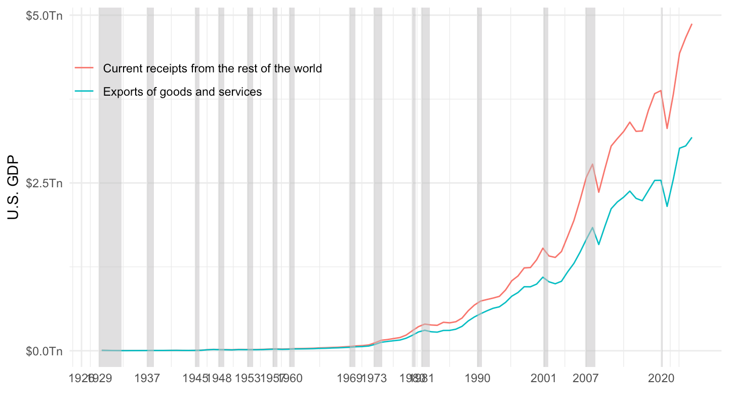
plot_log <- plot_linear +
  geom_rect(data = nber_recessions |>
              filter(Peak > as.Date("1928-01-01")),
            aes(xmin = Peak, xmax = Trough, ymin = -Inf, ymax = +Inf),
            fill = 'grey', alpha = 0.5) +
  scale_y_log10(breaks = c(0.1, 0.2, 0.5, 1, 2, 5, 8, 10, 20),
                     labels = scales::dollar_format(accuracy = 0.1, suffix = "Tn"))

plot_log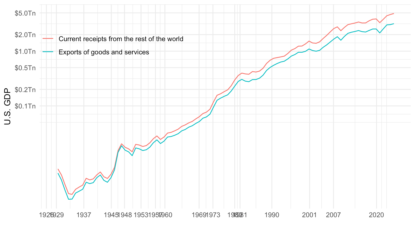
ggpubr::ggarrange(plot_linear + ggtitle("Linear Scale"),
                  plot_log + ggtitle("Log Scale") + ylab(""),
                  common.legend = T)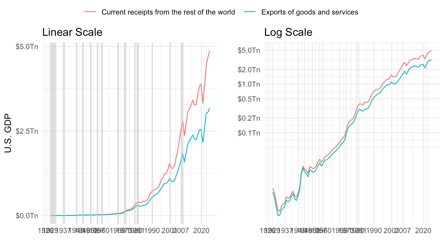
(ref:gdp-only) U.S. GDP (1929-2019).
T40100_A |>
  year_to_date() |>
  filter(LineNumber == 1) |>
  ggplot() + xlab("") + ylab("U.S. GDP") +
  geom_line(aes(x = date, y = DataValue/1000000)) +
  theme_minimal() +
  geom_rect(data = nber_recessions |>
              filter(Peak > as.Date("1928-01-01")),
            aes(xmin = Peak, xmax = Trough, ymin = -Inf, ymax = +Inf),
            fill = 'grey', alpha = 0.5) +
  theme(legend.title = element_blank(),
        legend.position = c(0.2, 0.8)) +
  scale_x_date(breaks = nber_recessions$Peak,
               labels = date_format("%Y")) +
  scale_y_continuous(breaks = 1*seq(0, 40, 2.5),
                     labels = scales::dollar_format(accuracy = 0.1, suffix = "Tn"))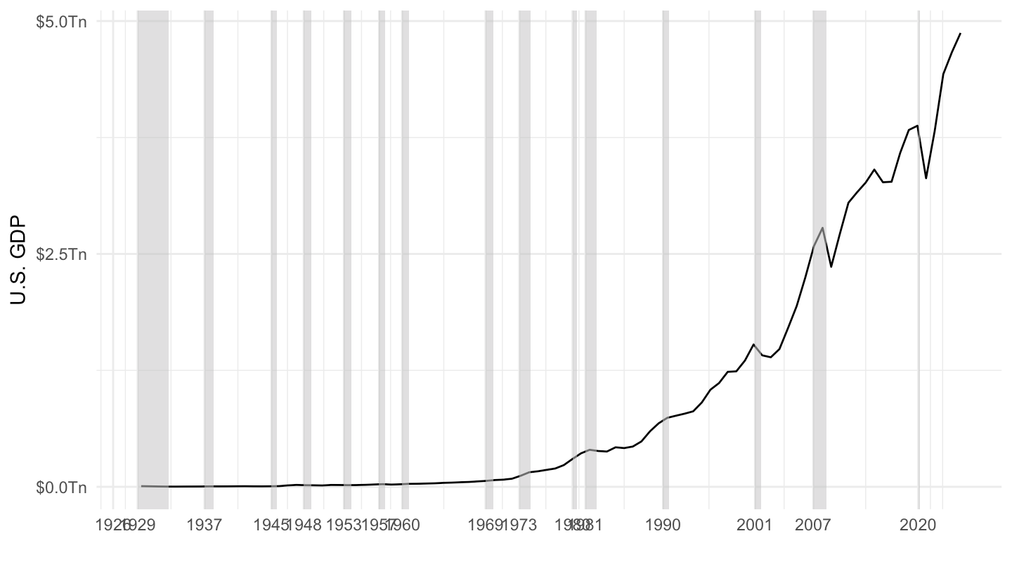
(ref:log-gdp-only) U.S. GDP (1929-2019) - Log Scale.
T40100_A |>
  year_to_date() |>
  filter(LineNumber == 1) |>
  ggplot() + xlab("") + ylab("U.S. GDP (Log Scale)") +
  geom_line(aes(x = date, y = DataValue/1000000)) + theme_minimal() +
  geom_rect(data = nber_recessions |>
              filter(Peak > as.Date("1928-01-01")),
            aes(xmin = Peak, xmax = Trough, ymin = 0, ymax = +Inf),
            fill = 'grey', alpha = 0.5) +
  theme(legend.title = element_blank(),
        legend.position = c(0.2, 0.8)) +
  scale_x_date(breaks = nber_recessions$Peak,
               labels = date_format("%Y")) +
  scale_y_log10(breaks = 20*2^seq(-9, 1, 1),
                labels = scales::dollar_format(accuracy = 0.1, suffix = "Tn"))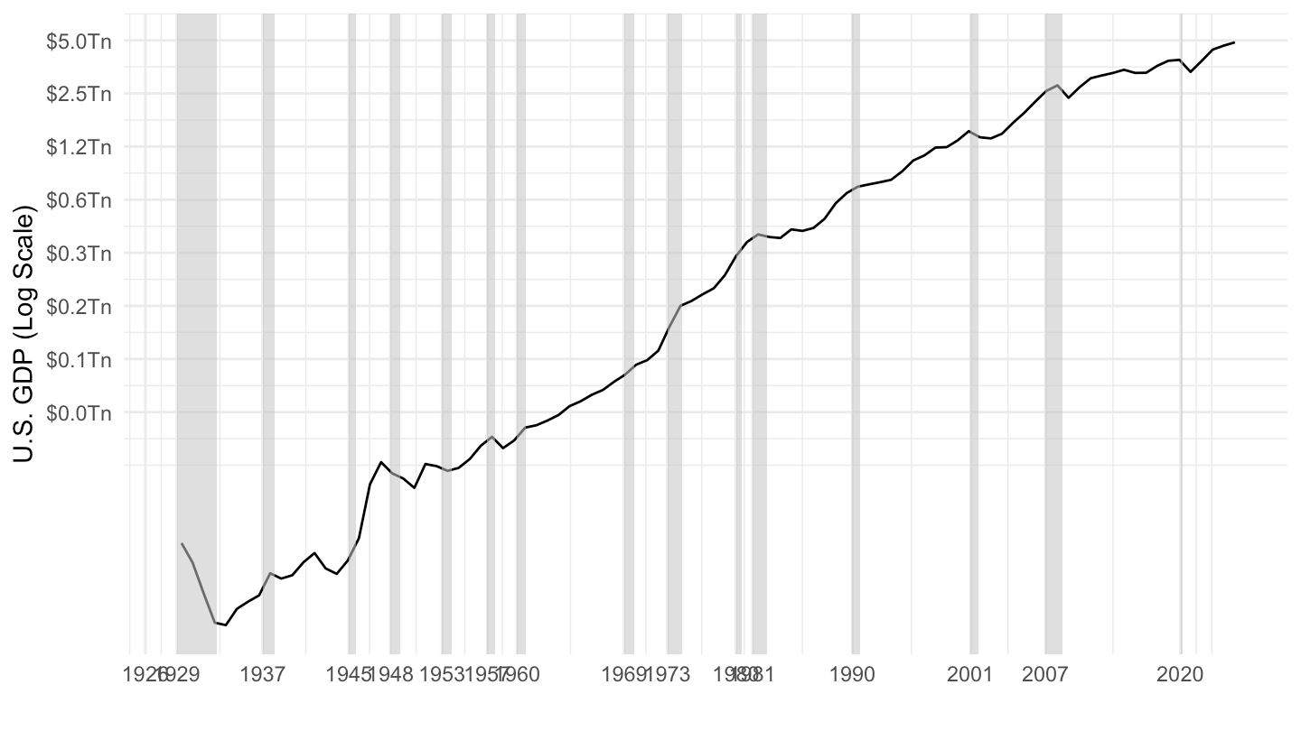
(ref:g-purchases) Government Purchases.
T40100_A |>
  year_to_date() |>
  filter(LineNumber %in% c(1, 22)) |>
  group_by(date) |>
  summarise(government_gdp = DataValue[LineNumber == 22]/DataValue[LineNumber == 1]) |>
  select(date, government_gdp) |>
  inner_join(gdp_real_A, by = "date") |>
  mutate(year = year(date),
         gdp_real_A_hp10000 = exp(hpfilter(log(gdp_real_A), freq = 10000)$trend),
         gdp_real_A_LLtrend = lm(log(gdp_real_A) ~ year) |> fitted() |> exp()) |>
  transmute(date,
            `Government Purchases (% of GDP)` = government_gdp,
            `Government Purchases (% of Log-Linear GDP Trend)` = government_gdp * gdp_real_A / gdp_real_A_LLtrend,
            `Government Purchases (% of HP GDP Trend)` = government_gdp * gdp_real_A / gdp_real_A_hp10000) |>
  gather(variable, value, -date) |>
  ggplot() + geom_line(aes(x = date, y = value, color = variable, linetype = variable)) + theme_minimal() +
  theme(legend.title = element_blank(),
        legend.position = c(0.4, 0.15)) +
  scale_color_manual(values = viridis(4)[1:3]) +
  geom_rect(data = nber_recessions |>
              filter(Peak > as.Date("1928-01-01")),
            aes(xmin = Peak, xmax = Trough, ymin = -Inf, ymax = +Inf),
            fill = 'grey', alpha = 0.5) +
  scale_x_date(breaks = nber_recessions$Peak,
               labels = date_format("%Y"),
               limits = as.Date(paste0(c(1947, 2019), "-01-01"))) +
  scale_y_continuous(breaks = seq(0.12, 0.29, 0.01),
                     labels = scales::percent_format(accuracy = 1),
                     limits = c(0.12, 0.29)) +
  xlab("") + ylab("Government Purchases (% of GDP)")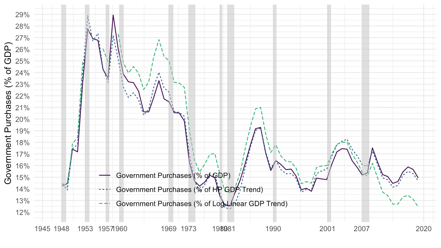
T40100_A |>
  year_to_date() |>
  filter(LineNumber %in% c(1, 13)) |>
  group_by(date) |>
  filter(n() == 2) |>
  summarise(government_gdp = DataValue[LineNumber == 13]/DataValue[LineNumber == 1]) |>
  select(date, government_gdp) |>
  inner_join(gdp_real_A, by = "date") |>
  mutate(year = year(date),
         gdp_real_A_hp10000 = log(gdp_real_A) |> hpfilter(freq = 10000) |> pluck("trend") |> exp(),
         gdp_real_A_LLtrend = lm(log(gdp_real_A) ~ year) |> fitted() |> exp()) |>
  transmute(date,
            `Residential Investment (% of GDP)` = government_gdp,
            `Residential Investment (% of Log-Linear GDP Trend)` = government_gdp * gdp_real_A / gdp_real_A_LLtrend,
            `Residential Investment (% of HP GDP Trend)` = government_gdp * gdp_real_A / gdp_real_A_hp10000) |>
  gather(variable, value, -date) |>
  ggplot() + geom_line(aes(x = date, y = value, color = variable, linetype = variable)) + theme_minimal() +
  theme(legend.title = element_blank(),
        legend.position = c(0.4, 0.15)) +
  scale_color_manual(values = viridis(4)[1:3]) +
  geom_rect(data = nber_recessions |>
              filter(Peak > as.Date("1928-01-01")),
            aes(xmin = Peak, xmax = Trough, ymin = -Inf, ymax = +Inf),
            fill = 'grey', alpha = 0.5) +
  scale_x_date(breaks = nber_recessions$Peak,
               labels = date_format("%Y"),
               limits = as.Date(paste0(c(1947, 2019), "-01-01"))) +
  scale_y_continuous(breaks = seq(0, 0.29, 0.01),
                     labels = scales::percent_format(accuracy = 1)) +
  xlab("") + ylab("Government Purchases (% of GDP)")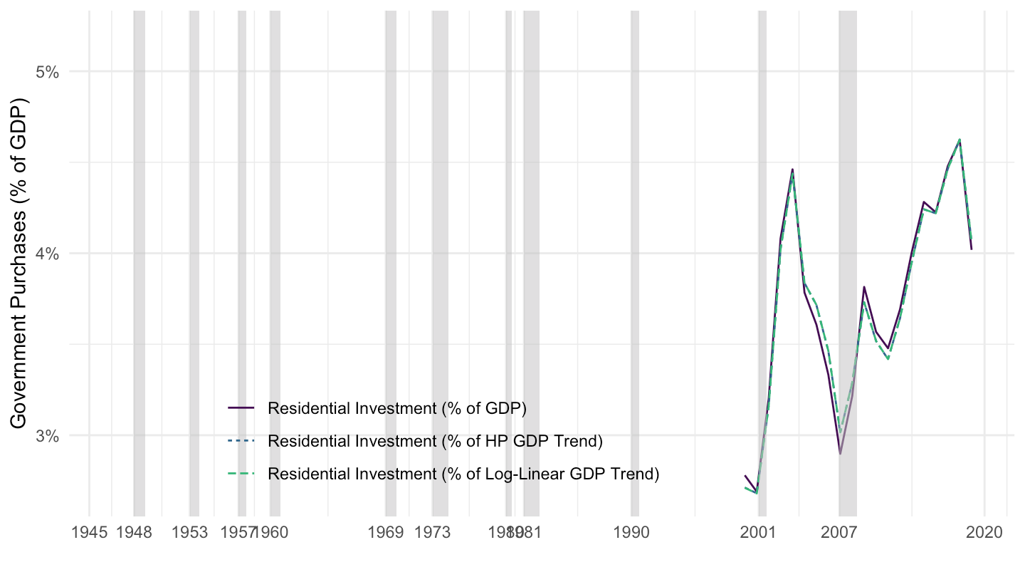
T40100_A |>
  year_to_date() |>
  filter(LineNumber %in% c(1, 15)) |>
  group_by(date) |>
  filter(n() == 2) |>
  summarise(net_exports_gdp = DataValue[LineNumber == 15]/DataValue[LineNumber == 1]) |>
  select(date, net_exports_gdp) |>
  inner_join(gdp_real_A, by = "date") |>
  mutate(year = year(date),
         gdp_real_A_hp10000 = log(gdp_real_A) |> hpfilter(freq = 10000) |> pluck("trend") |> exp(),
         gdp_real_A_LLtrend = lm(log(gdp_real_A) ~ year) |> fitted() |> exp()) |>
  transmute(date,
            `Net Exports (% of GDP)` = net_exports_gdp,
            `Net Exports (% of Log-Linear GDP Trend)` = net_exports_gdp * gdp_real_A / gdp_real_A_LLtrend,
            `Net Exports (% of HP GDP Trend)` = net_exports_gdp * gdp_real_A / gdp_real_A_hp10000) |>
  gather(variable, value, -date) |>
  ggplot() + theme_minimal() + xlab("") + ylab("Net Exports (% of GDP)") +
  geom_line(aes(x = date, y = value, color = variable, linetype = variable)) +
  geom_hline(yintercept = 0, linetype = "dashed",  color = "black") +
  scale_color_manual(values = viridis(4)[1:3]) +
  theme(legend.title = element_blank(),
        legend.position = c(0.75, 0.85)) +
  scale_x_date(breaks = seq(1920, 2100, 5) |> paste0("-01-01") |> as.Date(),
               labels = date_format("%Y")) +
  scale_y_continuous(breaks = seq(-0.06, 0.05, 0.01),
                     labels = scales::percent_format(accuracy = 1))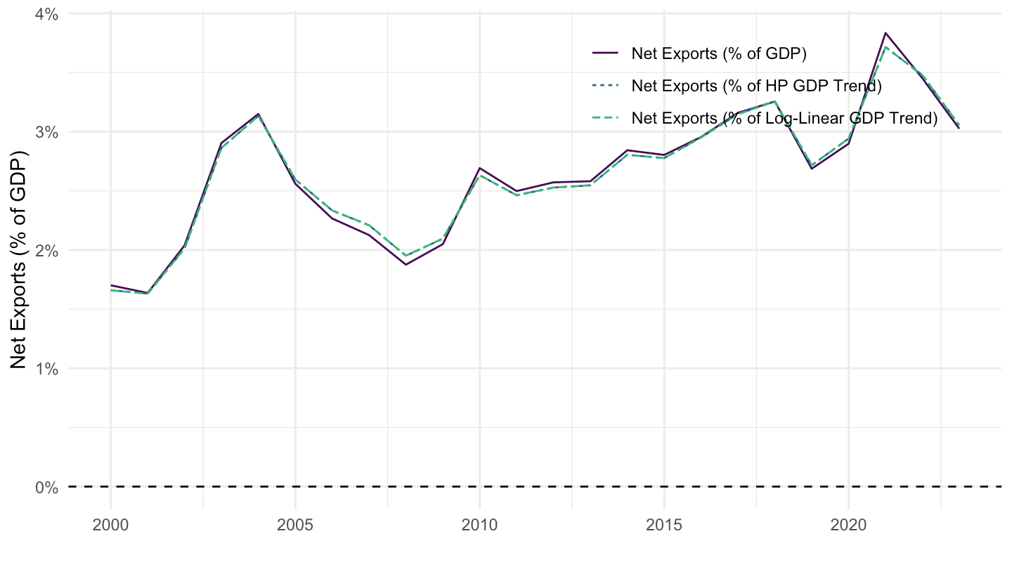
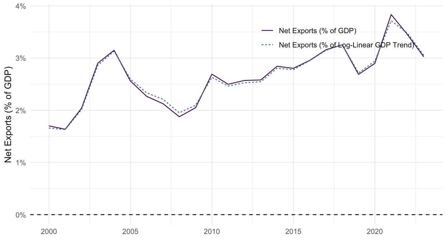
T40100_A |>
  year_to_date() |>
  filter(LineNumber %in% c(1, 15)) |>
  group_by(date) |>
  filter(n() == 2) |>
  summarise(net_exports_gdp = DataValue[LineNumber == 15]/DataValue[LineNumber == 1]) |>
  select(date, net_exports_gdp) |>
  inner_join(gdp_real_A, by = "date") |>
  mutate(year = year(date),
         gdp_real_A_LLtrend = exp(fitted(lm(log(gdp_real_A) ~ year)))) |>
  transmute(date,
            `Net Exports (% of GDP)` = net_exports_gdp,
            `Net Exports (% of Log-Linear GDP Trend)` = net_exports_gdp * gdp_real_A / gdp_real_A_LLtrend) |>
  gather(variable, value, -date) |>
  ggplot() + theme_minimal() + xlab("") + ylab("Net Exports (% of GDP)") +
  geom_line(aes(x = date, y = value, color = variable, linetype = variable)) +
  geom_hline(yintercept = 0, linetype = "dashed",  color = "black") +
  scale_color_manual(values = viridis(4)[1:3]) +
  theme(legend.title = element_blank(),
        legend.position = c(0.75, 0.85)) +
  scale_x_date(breaks = seq(1920, 2100, 5) |> paste0("-01-01") |> as.Date(),
               labels = date_format("%Y")) +
  scale_y_continuous(breaks = seq(-0.06, 0.05, 0.01),
                     labels = scales::percent_format(accuracy = 1))