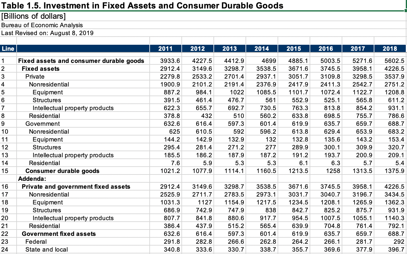
Table 1.5. Investment in Fixed Assets and Consumer Durable Goods (A) - FAAt105

Data - BEA

Layout

• Fixed Assets Website. html

Private vs Public Investment

Smoothed

FAAt105 %>%
  year_to_date %>%
  filter(LineNumber %in% c(3, 9)) %>%
  rename(variable = LineDescription) %>%
  left_join(gdp_adjustment, by = "date") %>%
  mutate(value = `Real GDP / Real GDP Trend (Log Linear)` * DataValue / GDP) %>%
  filter(!is.na(value)) %>%
  ggplot + geom_line(aes(x = date, y = value, color = variable)) + 
  ylab("% of GDP") + xlab("") + 
  theme_minimal()+
  geom_rect(data = nber_recessions %>%
              filter(Peak > as.Date("1927-01-01")),
            aes(xmin = Peak, xmax = Trough, ymin = -Inf, ymax = +Inf), 
            fill = 'grey', alpha = 0.5) +
  scale_x_date(breaks = nber_recessions$Peak,
               labels = date_format("%y")) + 
  scale_y_continuous(breaks = 0.01*seq(0, 40, 1),
                     labels = scales::percent_format(accuracy = 1)) + 
  theme(legend.position = c(0.1, 0.85),
        legend.title = element_blank(),
        legend.text = element_text(size = 8),
        legend.key.size = unit(0.9, 'lines'))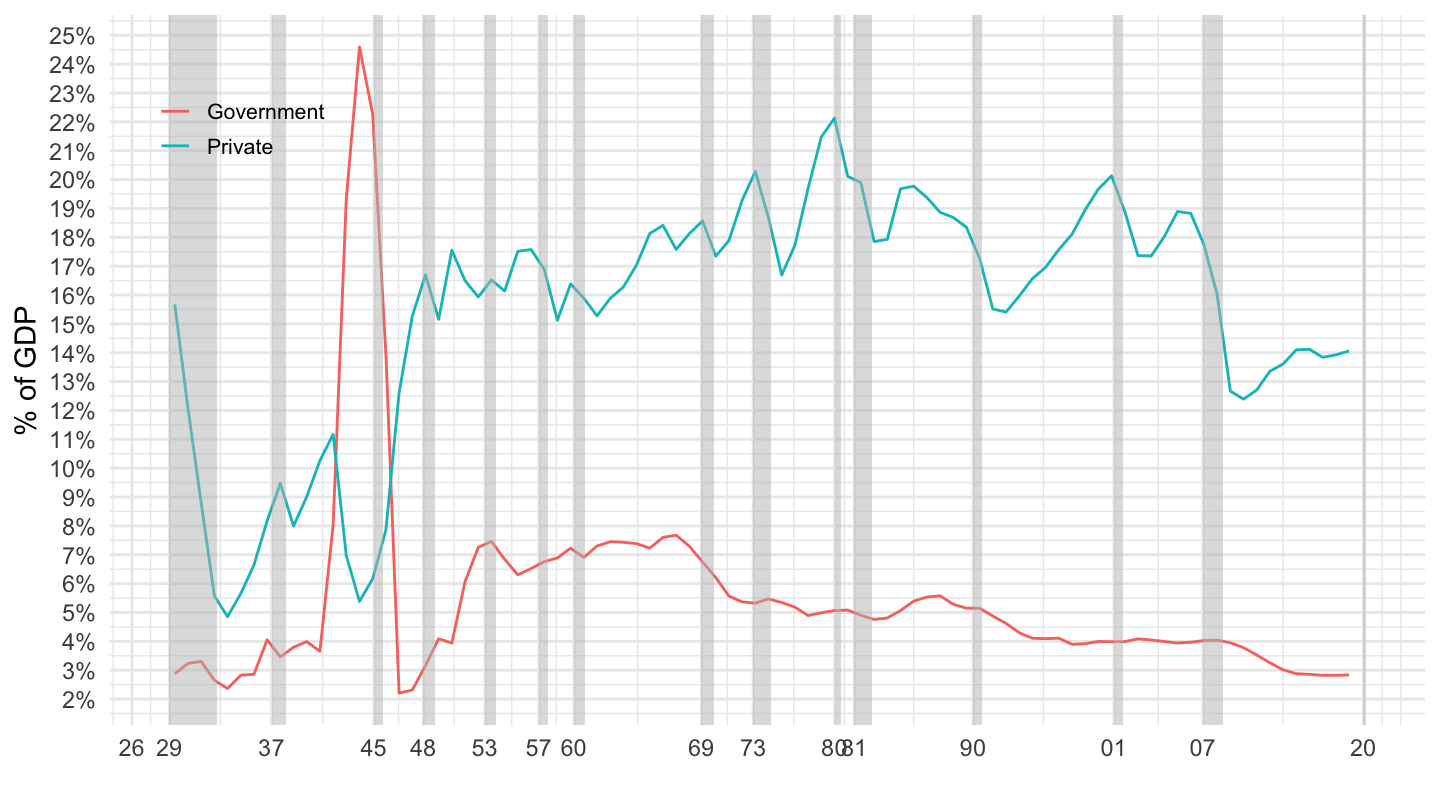

% of GDP

FAAt105 %>%
  year_to_date %>%
  filter(LineNumber %in% c(3, 9)) %>%
  rename(variable = LineDescription) %>%
  left_join(gdp_A, by = "date") %>%
  mutate(value = DataValue / value) %>%
  filter(!is.na(value)) %>%
  ggplot + geom_line(aes(x = date, y = value, color = variable)) + 
  ylab("% of GDP") + xlab("") + 
  theme_minimal()+
  geom_rect(data = nber_recessions %>%
              filter(Peak > as.Date("1927-01-01")),
            aes(xmin = Peak, xmax = Trough, ymin = -Inf, ymax = +Inf), 
            fill = 'grey', alpha = 0.5) +
  scale_x_date(breaks = nber_recessions$Peak,
               labels = date_format("%y")) + 
  scale_y_continuous(breaks = 0.01*seq(0, 40, 1),
                     labels = scales::percent_format(accuracy = 1)) + 
  theme(legend.position = c(0.1, 0.85),
        legend.title = element_blank(),
        legend.text = element_text(size = 8),
        legend.key.size = unit(0.9, 'lines'))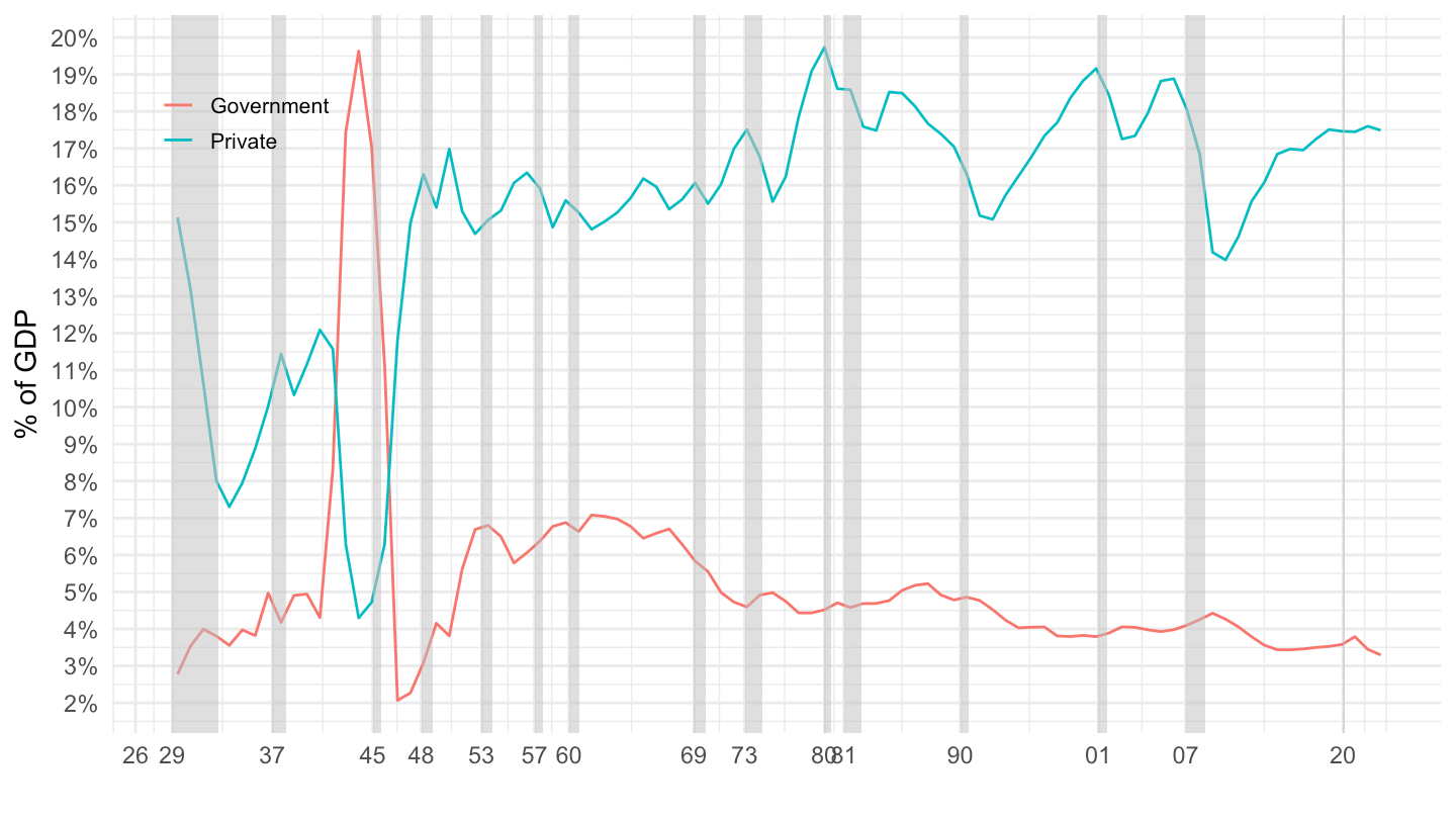

Types of investment

Smoothed

FAAt105 %>%
  year_to_date %>%
  filter(LineNumber %in% c(5, 6, 8, 15)) %>%
  rename(variable = LineDescription) %>%
  left_join(gdp_adjustment, by = "date") %>%
  mutate(value = `Real GDP / Real GDP Trend (Log Linear)` * DataValue / GDP) %>%
  filter(!is.na(value)) %>%
  ggplot + geom_line(aes(x = date, y = value, color = variable)) +
  ylab("% of GDP") + xlab("") + 
  theme_minimal()+
  geom_rect(data = nber_recessions %>%
              filter(Peak > as.Date("1927-01-01")),
            aes(xmin = Peak, xmax = Trough, ymin = -Inf, ymax = +Inf), 
            fill = 'grey', alpha = 0.5) +
  scale_x_date(breaks = nber_recessions$Peak,
               labels = date_format("%y")) + 
  scale_y_continuous(breaks = 0.01*seq(0, 15, 1),
                     labels = scales::percent_format(accuracy = 1)) + 
  theme(legend.position = c(0.45, 0.15),
        legend.title = element_blank(),
        legend.text = element_text(size = 8),
        legend.key.size = unit(0.9, 'lines'))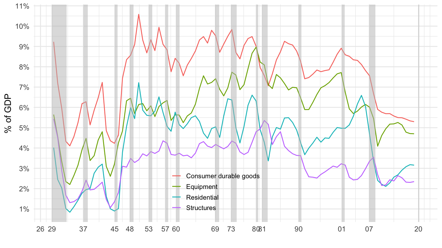

% of GDP

FAAt105 %>%
  year_to_date %>%
  filter(LineNumber %in% c(5, 6, 8, 15)) %>%
  rename(variable = LineDescription) %>%
  left_join(gdp_A, by = "date") %>%
  mutate(value = DataValue / value) %>%
  filter(!is.na(value)) %>%
  ggplot + geom_line(aes(x = date, y = value, color = variable)) +
  ylab("% of GDP") + xlab("") + 
  theme_minimal()+
  geom_rect(data = nber_recessions %>%
              filter(Peak > as.Date("1927-01-01")),
            aes(xmin = Peak, xmax = Trough, ymin = -Inf, ymax = +Inf), 
            fill = 'grey', alpha = 0.5) +
  scale_x_date(breaks = nber_recessions$Peak,
               labels = date_format("%y")) + 
  scale_y_continuous(breaks = 0.01*seq(0, 15, 1),
                     labels = scales::percent_format(accuracy = 1)) + 
  theme(legend.position = c(0.45, 0.15),
        legend.title = element_blank(),
        legend.text = element_text(size = 8),
        legend.key.size = unit(0.9, 'lines'))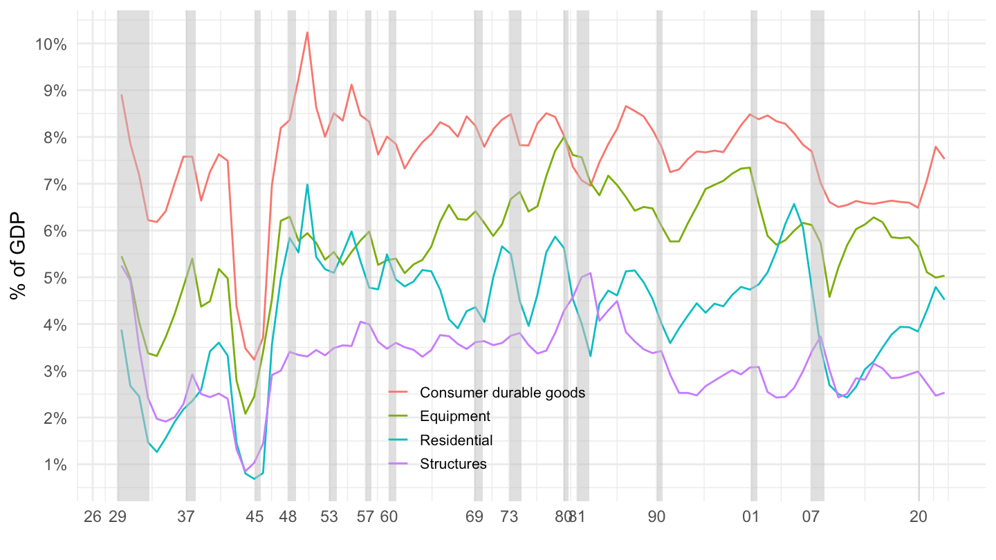

Ex 2: 1938, 1958, 1978, 1998, 2018 Table

Percent

FAAt105 %>%
  year_to_date %>%
  mutate(year = year(date)) %>%
  filter(year %in% c(1938, 1958, 1978, 1998, 2018)) %>%
  group_by(year) %>%
  mutate(value = round(100*DataValue/DataValue[1], 1)) %>%
  ungroup %>%
  select(LineNumber, LineDescription, year, value) %>%
  spread(year, value) %>%
  {if (is_html_output()) datatable(., filter = 'top', rownames = F) else .}

Billions

FAAt105 %>%
  year_to_date %>%
  mutate(year = year(date)) %>%
  filter(year %in% c(1938, 1958, 1978, 1998, 2018)) %>%
  group_by(year) %>%
  mutate(DataValue = round(DataValue)) %>%
  ungroup %>%
  select(LineNumber, LineDescription, year, DataValue) %>%
  spread(year, DataValue) %>%
  {if (is_html_output()) datatable(., filter = 'top', rownames = F) else .}