Indicateur de salaires négociés - INW

Données - BDF

🇬🇧 English version

Last observation: Q2 2026 (N = 22)

First observation: Q1 2006 (N = 1)

Last data update: 09 oct. 2026, 22:54

Last compile: 09 oct. 2026, 23:58

Structure

FREQ

REF_AREA

ADJUSTMENT

BCS_CONCEPT

BCS_CLASS

DATA_PROVIDER

TRANSFORMATION

UNIT_MEASURE

UNIT

UNIT_MULT

DECIMALS

Graphiques

Salaires négociés : branches, entreprises, Smic, inflation, SMPT

noms1 <- c(`000000` = "Salaires négociés (branches)", FR_000100 = "Accords d'entreprise (hausse moyenne)", FR_000200 = "Smic",
           FR_000300 = "Salaire moyen par tête", FR_000400 = "Inflation (IPC)")
INW |>
  mutate(code = sub("\\.FR2\\.GY\\.IX$", "", sub("^INW\\.Q\\.FR\\.N\\.INWR\\.", "", variable))) |>
  filter(code %in% names(noms1), date >= as.Date("2018-01-01")) |>
  mutate(serie = factor(noms1[code], levels = noms1)) |>
  arrange(date) |>
  ggplot(aes(x = date, y = value, color = serie)) + geom_line(linewidth = 0.9) +
  geom_hline(yintercept = 0, linetype = "dashed") +
  xlab("") + ylab("Glissement annuel") + theme_minimal() +
  scale_x_date(breaks = seq(2018, 2100, 1) |> paste0("-01-01") |> as.Date(),
               labels = date_format("%Y")) +
  scale_y_continuous(labels = scales::percent_format(accuracy = 1, scale = 1)) +
  guides(color = guide_legend(nrow = 2)) +
  theme(legend.position = "bottom", legend.title = element_blank())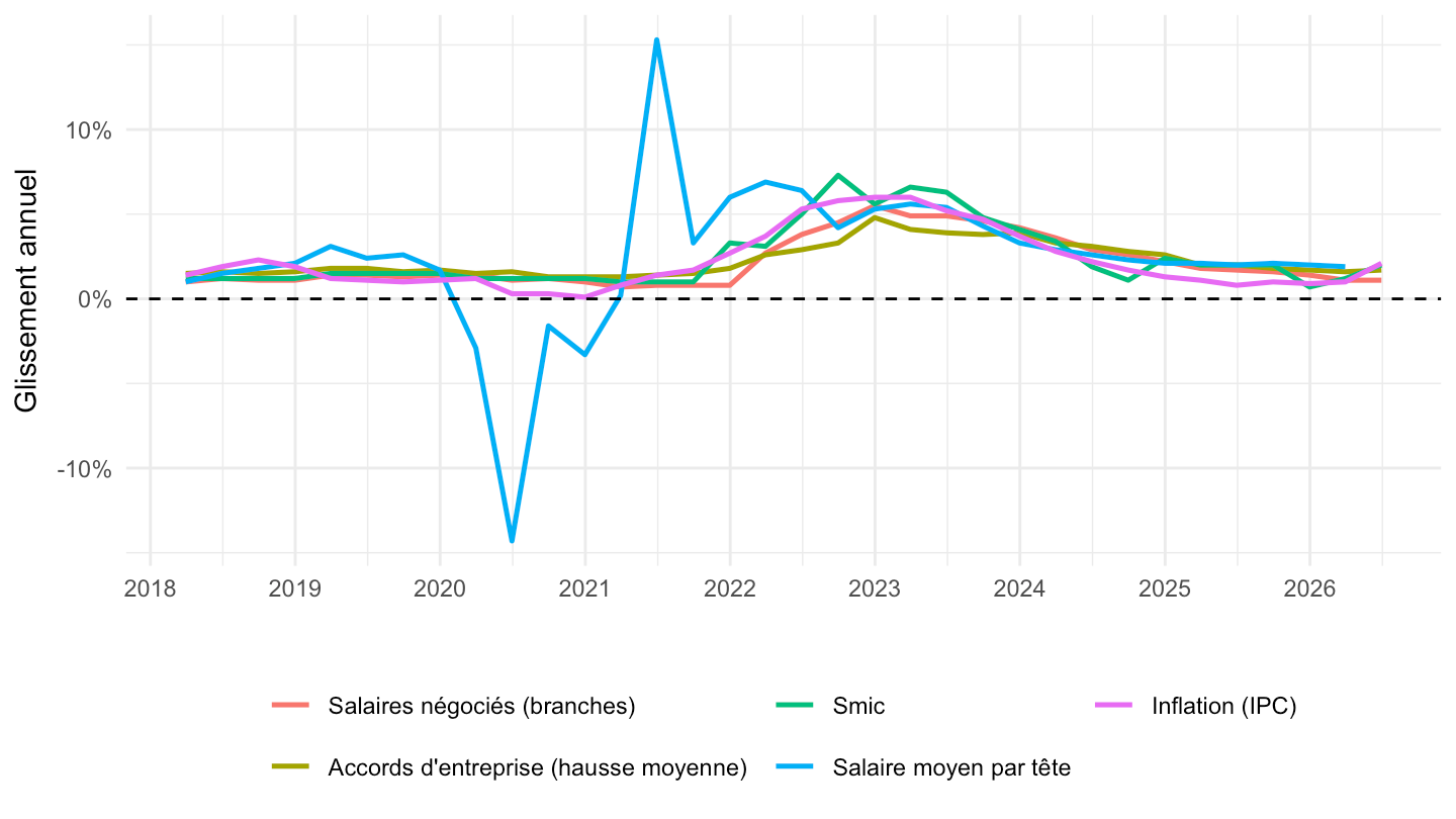

Accords de branche selon le niveau du minimum (en multiples du Smic)

noms2 <- c(FR_000001 = "< 1,05 Smic", FR_000002 = "1,05 – 1,2 Smic",
           FR_000003 = "1,2 – 1,6 Smic", FR_000004 = "> 1,6 Smic")
INW |>
  mutate(code = sub("\\.FR2\\.GY\\.IX$", "", sub("^INW\\.Q\\.FR\\.N\\.INWR\\.", "", variable))) |>
  filter(code %in% names(noms2)) |>
  mutate(serie = factor(noms2[code], levels = noms2)) |>
  arrange(date) |>
  ggplot(aes(x = date, y = value, color = serie)) + geom_line(linewidth = 0.9) +
  xlab("") + ylab("Glissement annuel") + theme_minimal() +
  scale_x_date(breaks = seq(2018, 2100, 1) |> paste0("-01-01") |> as.Date(),
               labels = date_format("%Y")) +
  scale_y_continuous(labels = scales::percent_format(accuracy = 1, scale = 1)) +
  guides(color = guide_legend(nrow = 2)) +
  theme(legend.position = "bottom", legend.title = element_blank())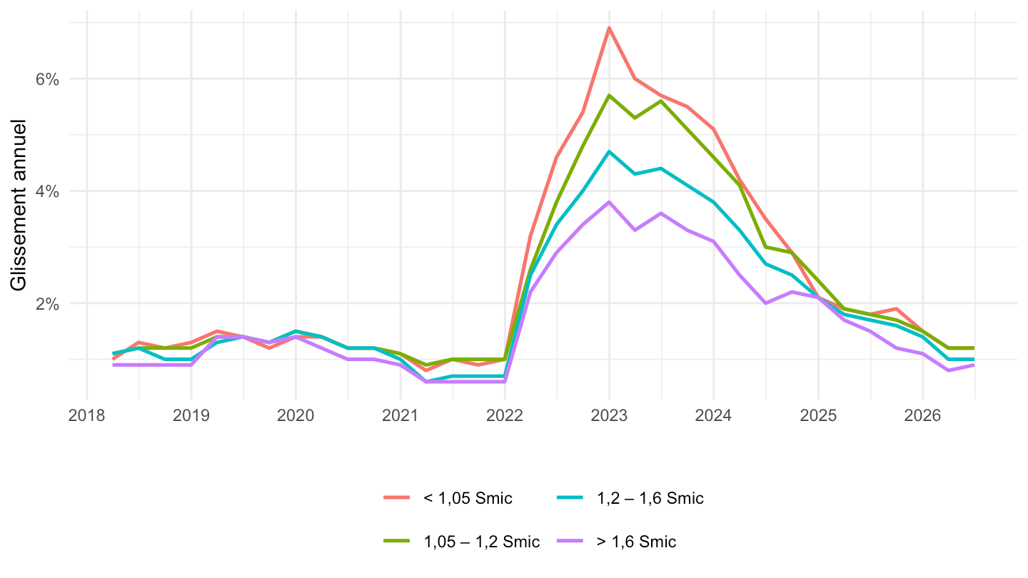

Distribution des hausses : accords de branche (%)

bins <- c("≤ 1 %", "1 – 2 %", "2 – 3 %", "3 – 4 %", "4 – 5 %", "5 – 6 %", "> 6 %")
distrib_plot <- function(codes) {
  names(codes) <- bins
  INW |>
    mutate(code = sub("\\.FR2\\.GY\\.IX$", "", sub("^INW\\.Q\\.FR\\.N\\.INWR\\.", "", variable))) |>
    filter(code %in% codes) |>
    mutate(classe = factor(names(codes)[match(code, codes)], levels = rev(bins))) |>
    ggplot(aes(x = date, y = value, fill = classe)) +
    geom_col(width = 70) +
    xlab("") + ylab("") + theme_minimal() +
    scale_fill_brewer(palette = "RdYlBu", direction = -1, breaks = bins) +
    scale_x_date(breaks = seq(2018, 2100, 1) |> paste0("-01-01") |> as.Date(),
                 labels = date_format("%Y")) +
    scale_y_continuous(labels = scales::percent_format(accuracy = 1, scale = 1)) +
    theme(legend.position = "bottom", legend.title = element_blank())
}
distrib_plot(c("FR_000011", "FR_000012", "FR_000013", "FR_000014", "FR_000015", "FR_000016", "FR_000017"))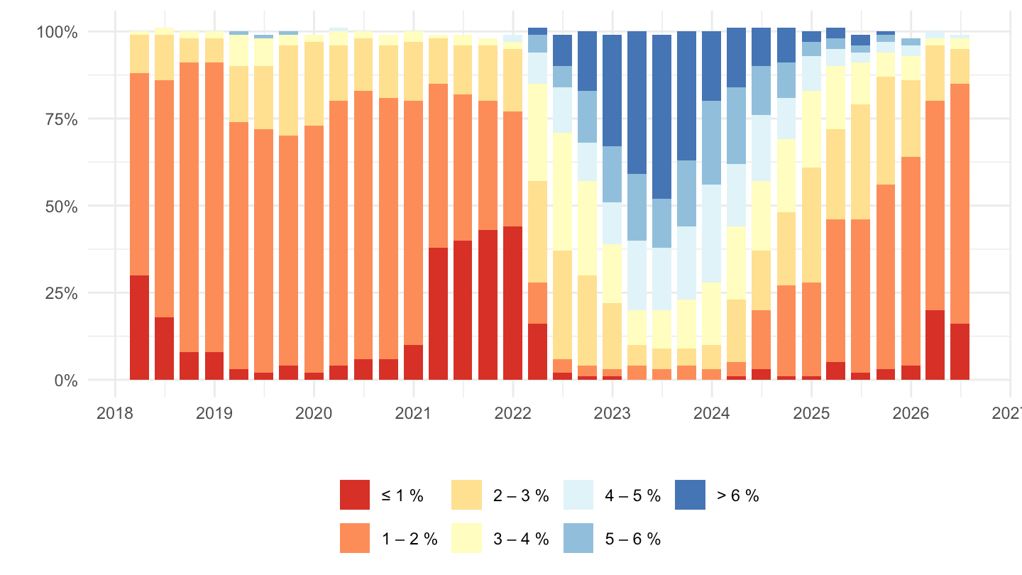

Distribution des hausses : accords d’entreprise (%)

distrib_plot(c("FR_000111", "FR_000112", "FR_000113", "FR_000114", "FR_000115", "FR_000116", "FR_000117"))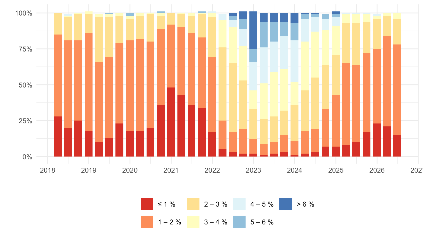

Séries

variable %>%
  {if (is_html_output()) datatable(., filter = 'top', rownames = F) else .}