Agrégats monétaires - Zone euro - BSI

Données - BDF

Auteur

François Geerolf

🇬🇧 English version

Info

Last observation: Mensuel: 30 jui 2026 (N = 554,868) · Trimestriel: 30 jui 2026 (N = 87,259)

First observation: Mensuel: 31 jan 1971 (N = 554,868) · Trimestriel: 31 mar 1993 (N = 87,259)

Last data update: 14 aoû 2026, 20:50. Last compile: 14 aoû 2026, 21:34

Structure

source	dataset	Title	Updated
bdf	DIREN	Observatoire des Entreprises	2026-08-10

Derniers

Dernier. html
Liste Données BDF Crédit aux particuliers. html
Crédits aux particuliers, Avril 2021. html / pdf
Crédits aux particuliers, Octobre 2021. html / pdf

LAST_DOWNLOAD

LAST_DOWNLOAD
2026-08-14

LAST_COMPILE

LAST_COMPILE
2026-08-14

Last

date	Nobs
2026-06-30	2127

Agrégats monétaires de la Zone euro (M1, M2, M3)

Taux de croissance annuel

Code

BSI |>
  
  filter(variable %in% c("BSI.M.U2.Y.V.M10.X.I.U2.2300.Z01.A",
                          "BSI.M.U2.Y.V.M20.X.I.U2.2300.Z01.A",
                          "BSI.M.U2.Y.V.M30.X.I.U2.2300.Z01.A")) |>
  mutate(Agregat = case_when(BS_ITEM == "M10" ~ "M1",
                              BS_ITEM == "M20" ~ "M2",
                              BS_ITEM == "M30" ~ "M3"),
         value = value/100) |>
  ggplot() + geom_line(aes(x = date, y = value, color = Agregat)) +
  geom_hline(yintercept = 0, linetype = "dashed", color = "black") +
  theme_minimal() + xlab("") + ylab("") +
  scale_x_date(breaks = seq(1960, 2100, 5) |> paste0("-01-01") |> as.Date(),
               labels = date_format("%Y")) +
  scale_y_continuous(labels = scales::percent_format(accuracy = 1)) +
  theme(legend.position = c(0.85, 0.85),
        legend.title = element_blank())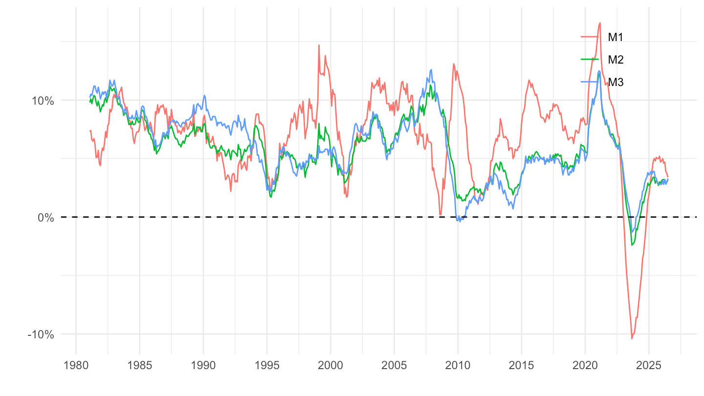

Depuis 2000

Code

BSI |>
  
  filter(variable %in% c("BSI.M.U2.Y.V.M10.X.I.U2.2300.Z01.A",
                          "BSI.M.U2.Y.V.M20.X.I.U2.2300.Z01.A",
                          "BSI.M.U2.Y.V.M30.X.I.U2.2300.Z01.A")) |>
  filter(date >= as.Date("2000-01-01")) |>
  mutate(Agregat = case_when(BS_ITEM == "M10" ~ "M1",
                              BS_ITEM == "M20" ~ "M2",
                              BS_ITEM == "M30" ~ "M3"),
         value = value/100) |>
  ggplot() + geom_line(aes(x = date, y = value, color = Agregat)) +
  geom_hline(yintercept = 0, linetype = "dashed", color = "black") +
  theme_minimal() + xlab("") + ylab("") +
  scale_x_date(breaks = seq(1960, 2100, 2) |> paste0("-01-01") |> as.Date(),
               labels = date_format("%Y")) +
  scale_y_continuous(labels = scales::percent_format(accuracy = 1)) +
  theme(legend.position = c(0.85, 0.85),
        legend.title = element_blank())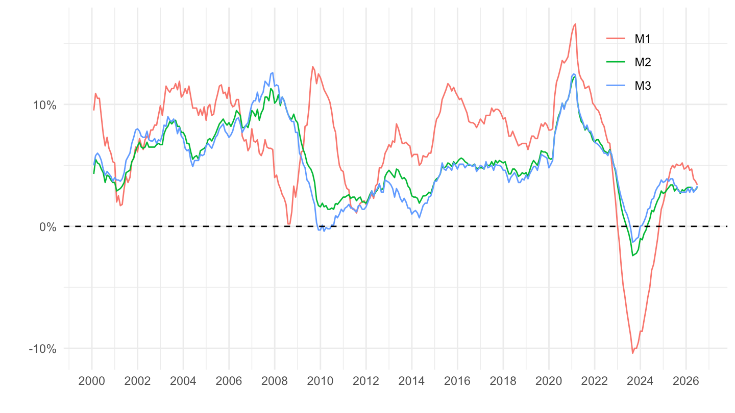

Encours (Mds €)

Code

BSI |>
  
  filter(variable %in% c("BSI.M.U2.Y.V.M10.X.1.U2.2300.Z01.E",
                          "BSI.M.U2.Y.V.M20.X.1.U2.2300.Z01.E",
                          "BSI.M.U2.Y.V.M30.X.1.U2.2300.Z01.E")) |>
  mutate(Agregat = case_when(BS_ITEM == "M10" ~ "M1",
                              BS_ITEM == "M20" ~ "M2",
                              BS_ITEM == "M30" ~ "M3"),
         value = value/1000) |>
  ggplot() + geom_line(aes(x = date, y = value, color = Agregat)) +
  theme_minimal() + xlab("") + ylab("") +
  scale_x_date(breaks = seq(1960, 2100, 5) |> paste0("-01-01") |> as.Date(),
               labels = date_format("%Y")) +
  scale_y_continuous(labels = dollar_format(accuracy = 1, prefix = "", suffix = " Mds€", big.mark = " ")) +
  theme(legend.position = c(0.15, 0.85),
        legend.title = element_blank())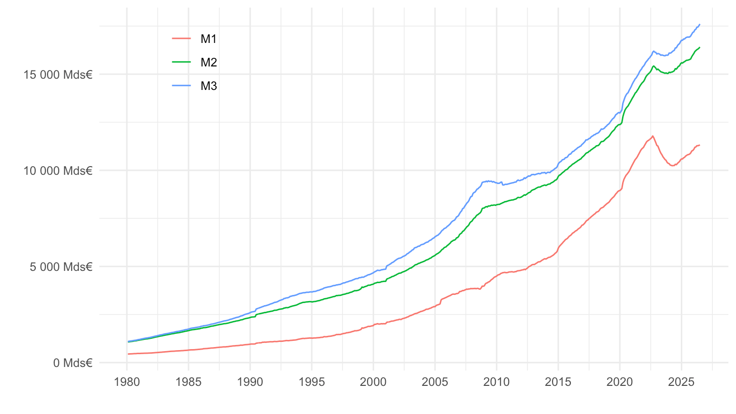

Crédits à l’habitat des ménages (taux de croissance annuel)

France, Allemagne, Italie, Espagne

Code

BSI |>
  
  filter(variable %in% c("BSI.M.FR.N.A.A22.A.I.U2.2250.Z01.A",
                          "BSI.M.DE.N.A.A22.A.I.U2.2250.Z01.A",
                          "BSI.M.IT.N.A.A22.A.I.U2.2250.Z01.A",
                          "BSI.M.ES.N.A.A22.A.I.U2.2250.Z01.A")) |>
  mutate(Ref_area = case_when(REF_AREA == "FR" ~ "France",
                               REF_AREA == "DE" ~ "Germany",
                               REF_AREA == "IT" ~ "Italy",
                               REF_AREA == "ES" ~ "Spain"),
         value = value/100) |>
  left_join(colors, by = c("Ref_area" = "country")) |>
  na.omit() |>
  ggplot() + geom_line(aes(x = date, y = value, color = color)) +
  geom_hline(yintercept = 0, linetype = "dashed", color = "black") +
  theme_minimal() + xlab("") + ylab("") + scale_color_identity() + add_4flags +
  scale_x_date(breaks = seq(1960, 2100, 2) |> paste0("-01-01") |> as.Date(),
               labels = date_format("%Y")) +
  scale_y_continuous(labels = scales::percent_format(accuracy = 1))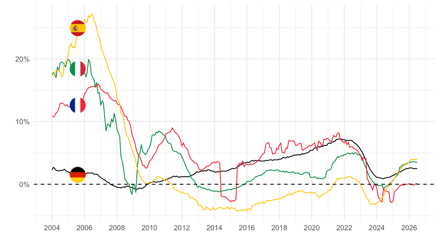

Dernier mois disponible

Code

BSI |>
  
  filter(variable %in% c("BSI.M.FR.N.A.A22.A.I.U2.2250.Z01.A",
                          "BSI.M.DE.N.A.A22.A.I.U2.2250.Z01.A",
                          "BSI.M.IT.N.A.A22.A.I.U2.2250.Z01.A",
                          "BSI.M.ES.N.A.A22.A.I.U2.2250.Z01.A")) |>
  filter(!is.na(value)) |>
  mutate(Ref_area = case_when(REF_AREA == "FR" ~ "France",
                               REF_AREA == "DE" ~ "Germany",
                               REF_AREA == "IT" ~ "Italy",
                               REF_AREA == "ES" ~ "Spain")) |>
  group_by(Ref_area) |>
  filter(date == max(date)) |>
  ungroup() |>
  select(Ref_area, date, value) |>
  arrange(desc(value)) |>
  print_table_conditional()

Ref_area	date	value
Spain	2026-06-30	3.9
Italy	2026-06-30	3.5
Germany	2026-06-30	2.5
France	2026-06-30	0.1