Output gap and potential growth, real-time vs. revised - vintages-output-gap

Data - AMECO

Last observation: 2027 (N = 328)

First observation: 1960 (N = 1968)

Last data update: 01 oct. 2026, 22:36

Last compile: 05 oct. 2026, 00:09

The output gap is not observed: it is re-estimated with every vintage. Black: latest vintage.

Output gap

Revisions, France, Germany, Italy, Spain

vintages |>
  filter(VAR == "AVGDGP", COU %in% countries_4) |>
  mutate(value = value / 100) |>
  plot_vintage_paths("Output gap (% of potential GDP)", from = 2000)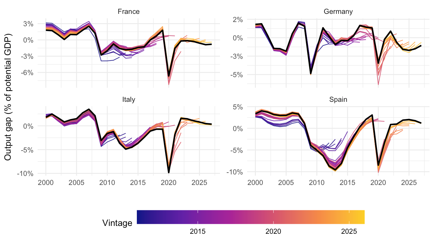

Real-time vs. revised

Estimate for year t in the autumn vintage of year t (real time), vs. the latest estimate.

og <- vintages |> filter(VAR == "AVGDGP", COU %in% countries_4) |> mutate(value = value / 100)
bind_rows(og |> filter(season == "autumn", year == vintage_year) |> mutate(estimate = "Real time (autumn of year t)"),
          og |> filter(vintage == latest_vintage) |> mutate(estimate = paste0("Latest (", vintage_label, ")"))) |>
  filter(year >= 2000, year <= 2025) |>
  ggplot(aes(x = date, y = value, color = estimate)) + theme_minimal() +
  geom_hline(yintercept = 0, linewidth = 0.3) + geom_line() + geom_point(size = 0.8) +
  facet_wrap(~COUNTRY) + xlab("") + ylab("Output gap (% of potential GDP)") +
  scale_color_manual(values = c("#d95f02", "black")) +
  scale_x_date(breaks = seq(1920, 2100, 5) |> paste0("-01-01") |> as.Date(), labels = date_format("%Y")) +
  scale_y_continuous(labels = percent_format(accuracy = 1)) +
  theme(legend.position = "bottom", legend.title = element_blank())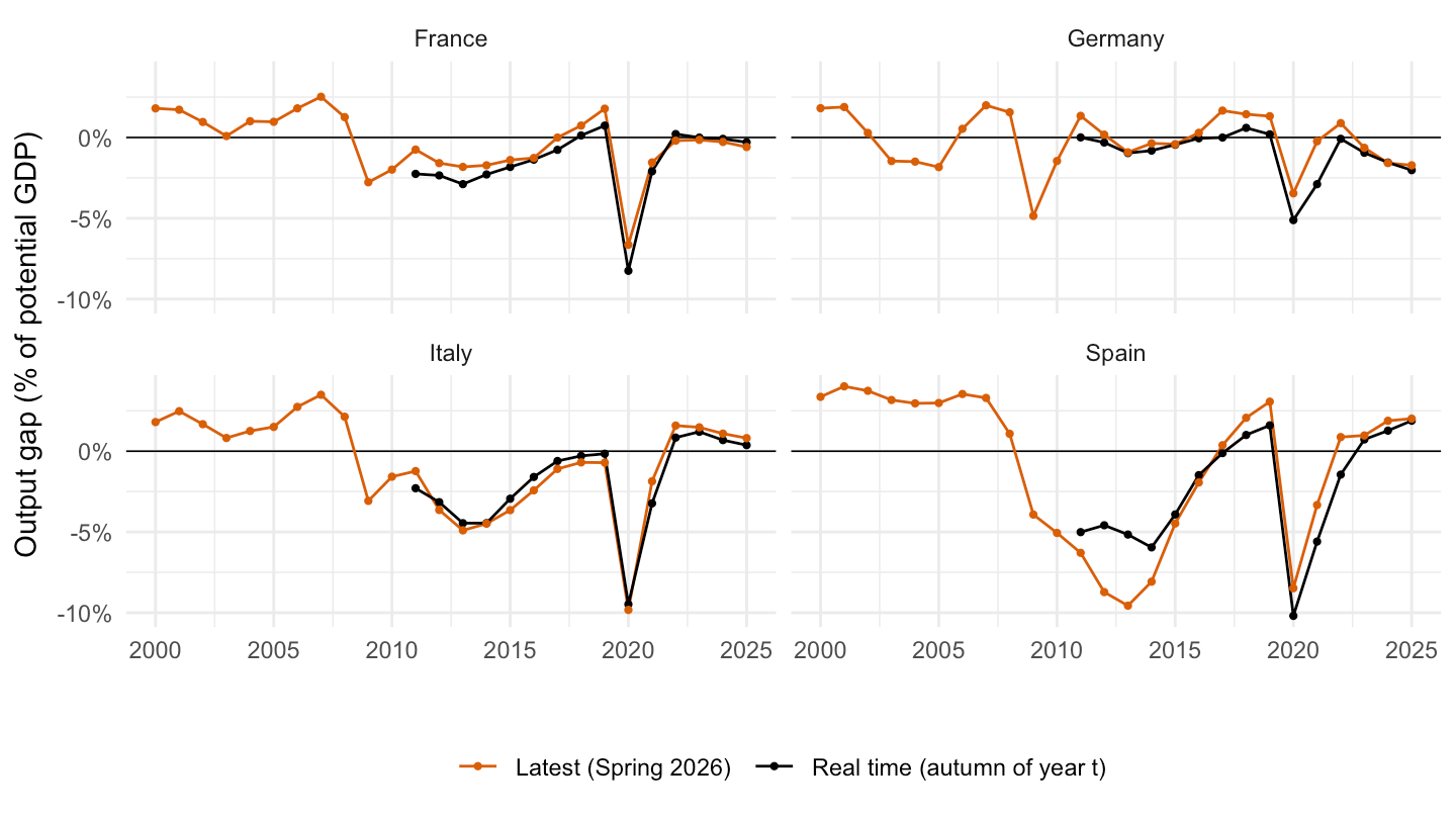

Real-time vs. revised: all countries (scatter)

og_all <- vintages |> filter(VAR == "AVGDGP") |> mutate(value = value / 100)
inner_join(og_all |> filter(season == "autumn", year == vintage_year) |> select(COUNTRY, year, rt = value),
           og_all |> filter(vintage == latest_vintage) |> select(COUNTRY, year, latest = value),
           by = c("COUNTRY", "year")) |>
  filter(year >= 2005, year <= 2024) |>
  ggplot(aes(x = rt, y = latest, color = year)) + theme_minimal() +
  geom_abline(slope = 1, intercept = 0, linetype = "dashed") +
  geom_point(alpha = 0.8) + scale_color_viridis_c(option = "plasma", end = 0.9) +
  xlab("Real-time estimate (autumn of year t)") + ylab("Latest estimate") +
  scale_x_continuous(labels = percent_format(accuracy = 1)) +
  scale_y_continuous(labels = percent_format(accuracy = 1))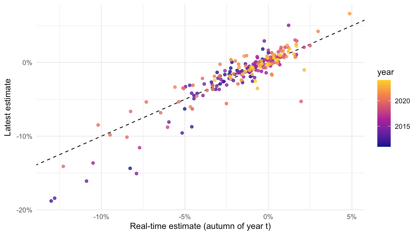

Potential growth

Revisions, France, Germany, Italy, Spain

potential_growth |>
  filter(COU %in% countries_4) |>
  plot_vintage_paths("Potential GDP growth", from = 2000, accuracy = 0.5)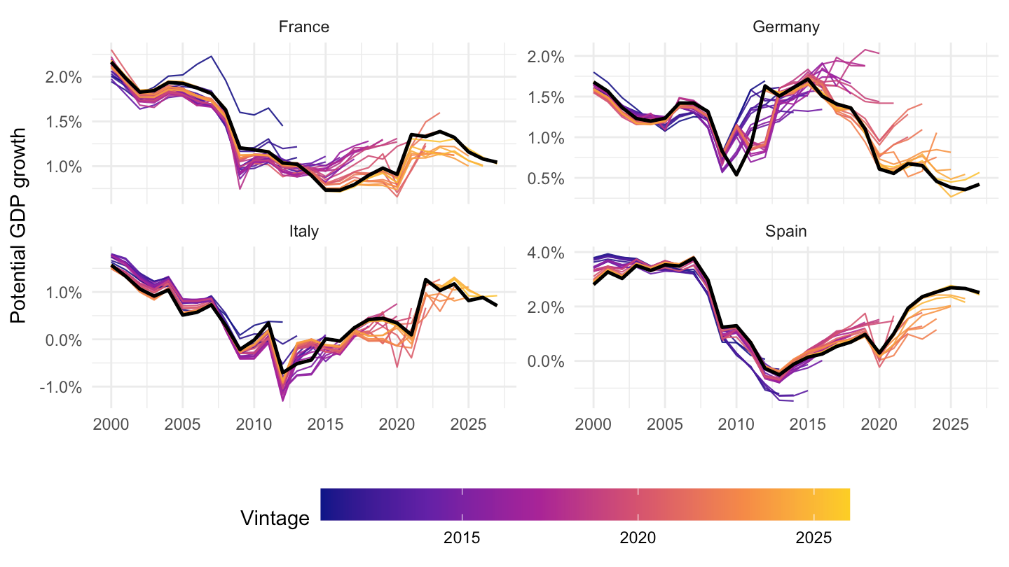

Potential growth in 2020, as seen over time

potential_growth |>
  filter(COU %in% c("FRA", "DEU", "ITA", "ESP", "GRC", "PRT")) |>
  plot_target_year(c(2015, 2020, 2025), "Potential GDP growth", accuracy = 0.5)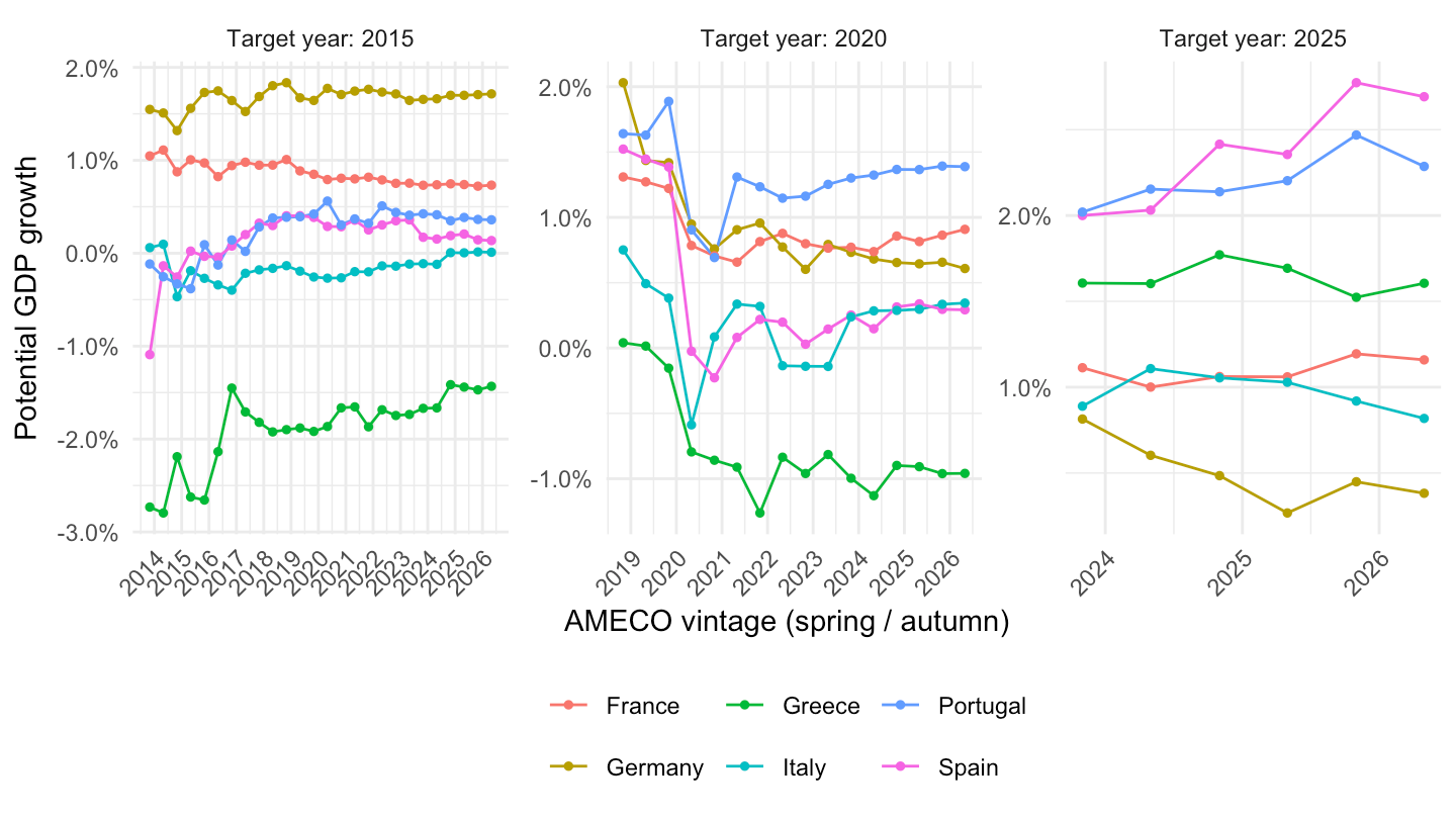

Structural primary balance

Revisions (since the 2014 vintages)

vintages |>
  filter(VAR == "UBLGBPS", COU %in% countries_4) |>
  mutate(value = value / 100) |>
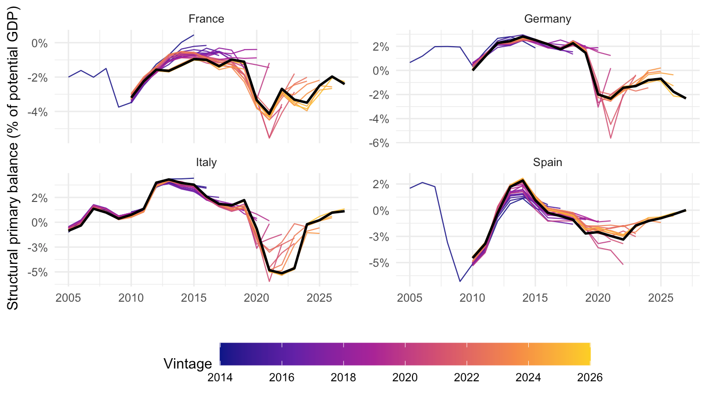
  plot_vintage_paths("Structural primary balance (% of potential GDP)", from = 2005, accuracy = 1)