Last observation: 2027 (N = 328)
First observation: 1960 (N = 1968)
Last data update: 01 oct. 2026, 22:36
Last compile: 24 oct. 2026, 00:03
Each AMECO vintage (spring: May, autumn: November) contains the European Commission’s forecasts. Real GDP growth is computed from the level series of each vintage. Black: latest vintage.
gdp_growth |>
  filter(COU %in% countries_4) |>
  plot_vintage_paths("Real GDP growth", from = 2015)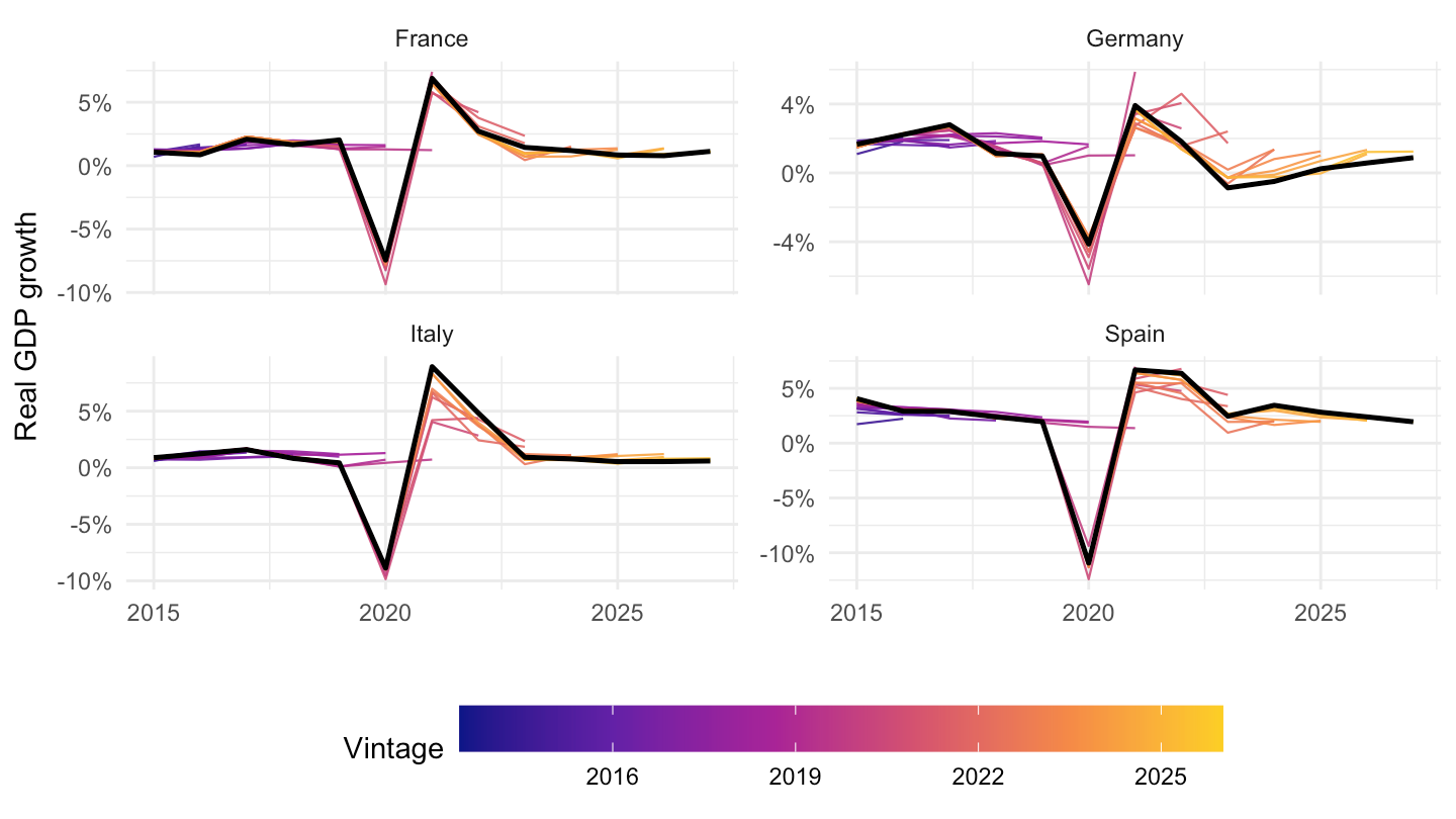
gdp_growth |>
  filter(COU %in% countries_4, !year %in% 2020:2021) |>
  plot_vintage_paths("Real GDP growth", from = 2017, accuracy = 0.5)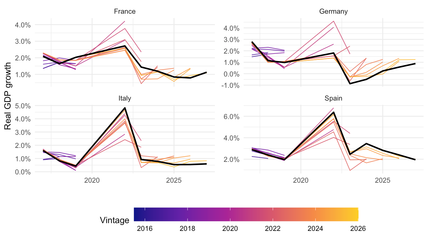
gdp_growth |>
  filter(COU %in% countries_4) |>
  plot_target_year(c(2020, 2022, 2023, 2025), "Real GDP growth")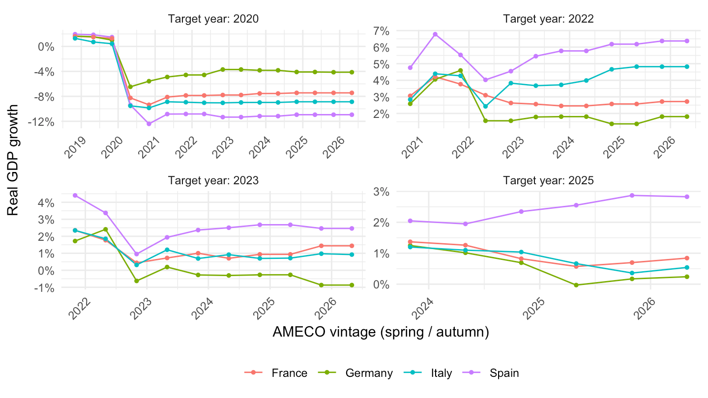
gdp_growth |>
  filter(COU %in% c("FRA", "DEU", "ITA", "ESP", "GRC", "PRT")) |>
  plot_target_year(c(2012, 2013, 2014), "Real GDP growth")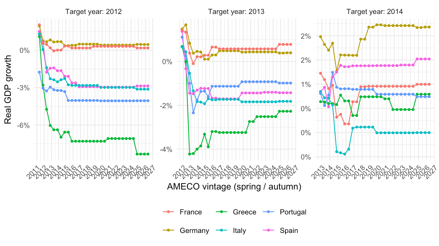
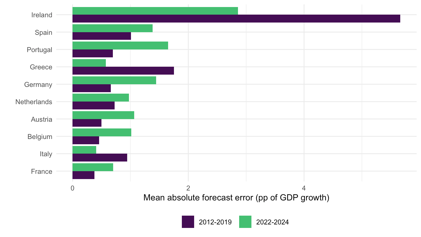
Latest vintage minus the autumn forecast made the previous year, in percentage points. Positive: growth turned out stronger than forecast.
gdp_growth |>
  filter(COU %in% countries_10) |>
  error_heatmap(lag_years = 1)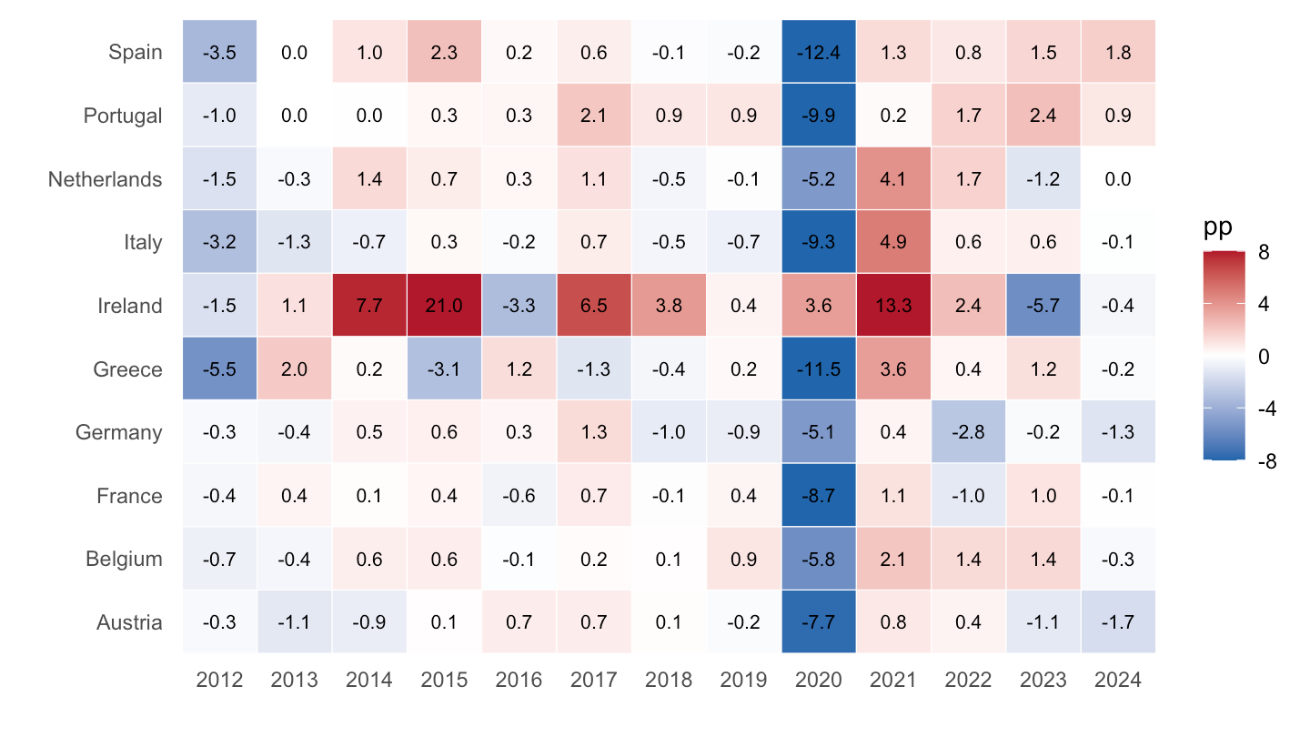
gdp_growth |>
  filter(COU %in% countries_10) |>
  mutate(vintage_year = vintage_year) |>
  error_heatmap(lag_years = 0, ref_season = "spring")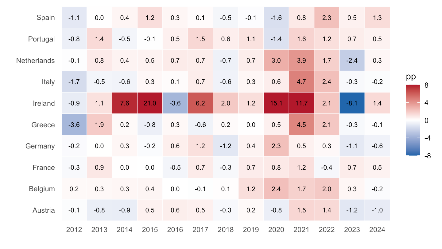
ref <- gdp_growth |>
  filter(season == "autumn", COU %in% countries_10) |>
  filter(year == vintage_year + 1) |>
  select(COUNTRY, year, forecast = value)
fin <- gdp_growth |> filter(vintage == latest_vintage) |> select(COUNTRY, year, latest = value)
inner_join(ref, fin, by = c("COUNTRY", "year")) |>
  mutate(period = case_when(year %in% 2012:2019 ~ "2012-2019",
                            year %in% 2022:2024 ~ "2022-2024")) |>
  filter(!is.na(period)) |>
  group_by(COUNTRY, period) |>
  summarise(MAE = mean(abs(latest - forecast)) * 100, .groups = "drop") |>
  ggplot(aes(x = reorder(COUNTRY, MAE), y = MAE, fill = period)) + theme_minimal() +
  geom_col(position = "dodge") + coord_flip() + xlab("") +
  ylab("Mean absolute forecast error (pp of GDP growth)") +
  scale_fill_viridis_d(end = 0.7) + theme(legend.position = "bottom", legend.title = element_blank())