Annual Macro-Economic database of the European COmmission (AMECO)
Data
Main Datasets
Info
- AMECO DATA FILE CODING pdf
In the AMECO data files, a series code such as EU27.1.0.0.0.NPTD consists of a country code at the beginning, the AMECO variable code at the end, and four numeric values representing, in order:
- TRN: Transformations over time
- AGG: Aggregation modes
- UNIT: Unit codes
- REF: Codes for relative performance
Labels for country and variable codes are included directly in the data file. The four numerical codes are explained in the following sections.
Other
Javascript
Flat
| id | Title | .RData | .html |
|---|---|---|---|
| api | AMECO's API | NA | [2025-08-24] |
| AVGDGP | Gap between actual and potential gross domestic product at 2015 reference levels - AVGDGP | 2023-10-05 | [2025-08-24] |
| AVGDGT | Gap between actual and trend gross domestic product at 2015 reference levels - AVGDGT | 2022-02-02 | [2025-08-24] |
| index-old | Annual Macro-Economic database of the European COmmission - AMECO | NA | [2025-08-24] |
| OVGDP | Potential gross domestic product at 2015 reference levels - OVGDP | 2021-07-04 | [2025-08-24] |
| PLCD | Nominal unit labour costs - total economy (Ratio of compensation per employee to real GDP per person employed.) - PLCD | 2022-02-02 | [2025-08-24] |
| PLCDQ | Nominal unit labour costs, total economy :- Performance relative to the rest of 37 industrial countries - PLCDQ | 2022-02-02 | [2025-08-24] |
| PLCM | Nominal unit labour costs - manufacturing industry - PLCM | 2021-07-01 | [2025-08-24] |
| PMGN | Price deflator imports of goods - PMGN | 2021-01-31 | [2025-08-24] |
| QLCD | Real unit labour costs - total economy (Ratio of compensation per employee to nominal GDP per person employed.) - QLCD | 2022-02-02 | [2025-08-24] |
| session6 | "Session 6 - R-markdown" | NA | [2025-08-24] |
| UBLGBPS | Structural balance of general government excluding interest :- Adjustment based on potential GDP Excessive deficit procedure - UBLGBPS | 2024-05-06 | [2025-08-24] |
| ZNAWRU | Non-accelerating wage rate of unemployment - ZNAWRU | 2024-10-24 | [2025-08-24] |
| ZUTN | Unemployment rate - total - Member States - definition EUROSTAT - ZUTN | 2021-07-04 | [2025-08-24] |
COU, COUNTRY
Code
ameco %>%
  group_by(COU, COUNTRY) %>%
  summarise(Nobs = n()) %>%
  mutate(Flag = gsub(" ", "-", str_to_lower(COUNTRY)),
         Flag = paste0('<img src="../../icon/flag/vsmall/', Flag, '.png" alt="Flag">')) %>%
  select(Flag, everything()) %>%
  {if (is_html_output()) datatable(., filter = 'top', rownames = F, escape = F) else .}
Output gap
France, Italy, Spain
Code
ameco %>%
  filter(VAR == "AVGDGP",
         COU %in% c("FRA", "ESP", "ITA")) %>%
  select(COUNTRY, date, value) %>%
  arrange(COUNTRY, date) %>%
  left_join(colors, c("COUNTRY" = "country")) %>%
  mutate(value = value / 100) %>%
  ggplot() + theme_minimal() + ylab("Output Gap (% of GDP)") + xlab("") +
  geom_line(aes(x = date, y = value, color = color)) +
  scale_color_identity() + add_3flags +
  scale_x_date(breaks = seq(1920, 2025, 5) %>% paste0("-01-01") %>% as.Date,
               labels = date_format("%y")) +
  theme(legend.position = "none") +
  scale_y_continuous(breaks = 0.01*seq(-60, 60, 1),
                     labels = scales::percent_format(accuracy = 1))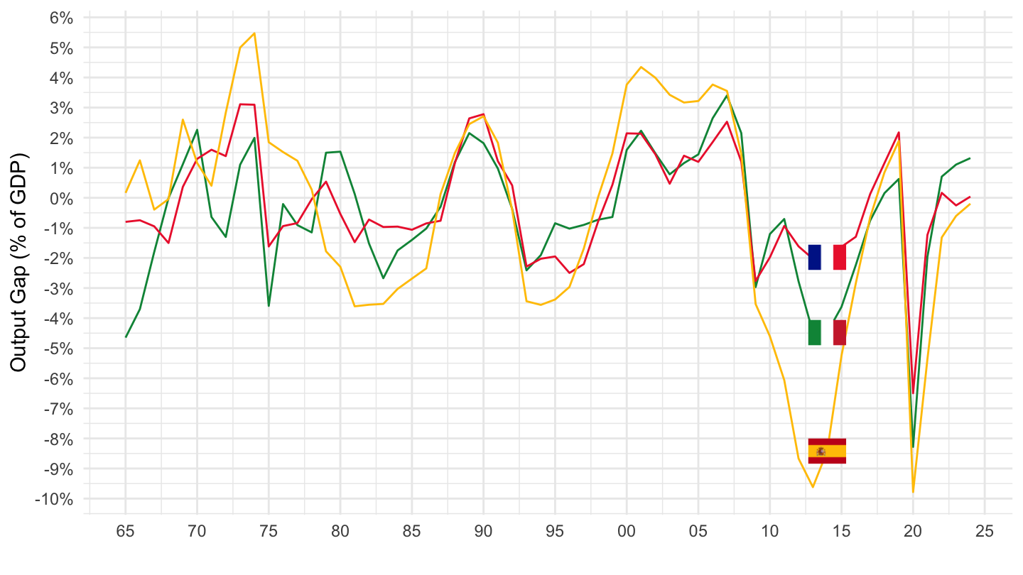
PLCDQ - Nominal unit labour costs: total economy :- Performance relative to the rest of 37 industrial countries
France, Germany
All
Code
ameco %>%
  filter(VAR == "PLCDQ",
         COU %in% c("FRA", "DEU"),
         CODE_4 == "30",
         CODE_5 == "437") %>%
  select(COUNTRY, date, value, CODE) %>%
  arrange(COUNTRY, date) %>%
  left_join(colors, c("COUNTRY" = "country")) %>%
  ggplot() + ylab("Nominal unit labour costs (total economy)") + xlab("") + theme_minimal() +
  geom_line(aes(x = date, y = value, color = color)) +
  scale_color_identity() + add_2flags +
  scale_x_date(breaks = seq(1920, 2025, 5) %>% paste0("-01-01") %>% as.Date,
               labels = date_format("%y")) +
  theme(legend.position = c(0.8, 0.9),
        legend.title = element_blank()) +
  scale_y_continuous(breaks = seq(-60, 300, 5))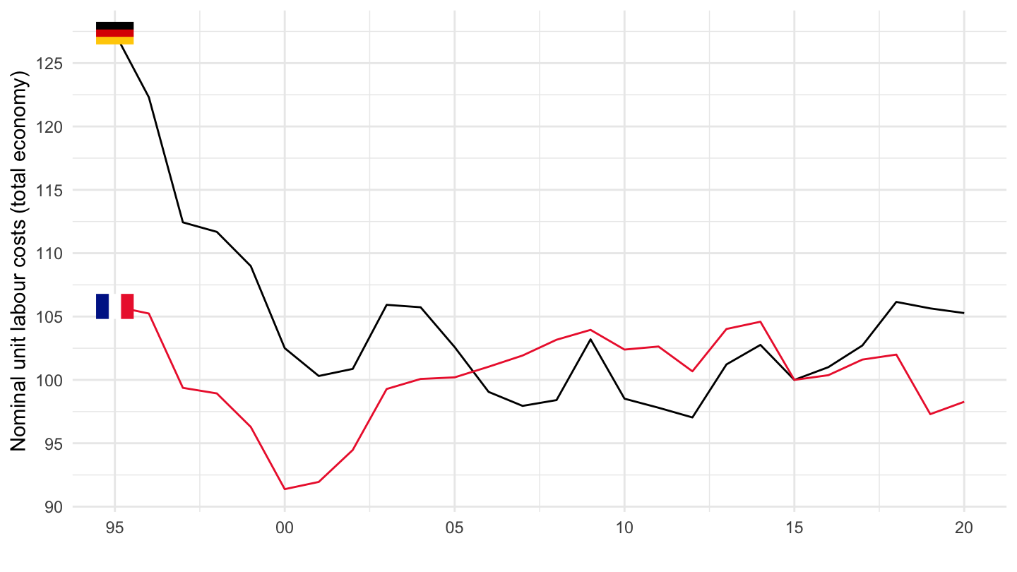
1995-
Code
ameco %>%
  filter(VAR == "PLCDQ",
         COU %in% c("FRA", "DEU"),
         CODE_4 == "30",
         CODE_5 == "437") %>%
  select(COUNTRY, date, value, CODE) %>%
  arrange(COUNTRY, date) %>%
  filter(date >= as.Date("1995-01-01")) %>%
  group_by(COUNTRY) %>%
  mutate(value = 100*value / value[date == as.Date("1995-01-01")]) %>%
  left_join(colors, c("COUNTRY" = "country")) %>%
  ggplot() + ylab("Nominal unit labour costs (total economy)") + xlab("") + theme_minimal() +
  geom_line(aes(x = date, y = value, color = color)) +
  scale_color_identity() + add_2flags +
  scale_x_date(breaks = seq(1920, 2025, 5) %>% paste0("-01-01") %>% as.Date,
               labels = date_format("%y")) +
  geom_vline(xintercept = as.Date("2011-01-01"),
             linetype= "dashed") +
  theme(legend.position = c(0.8, 0.9),
        legend.title = element_blank()) +
  scale_y_continuous(breaks = seq(-60, 300, 5))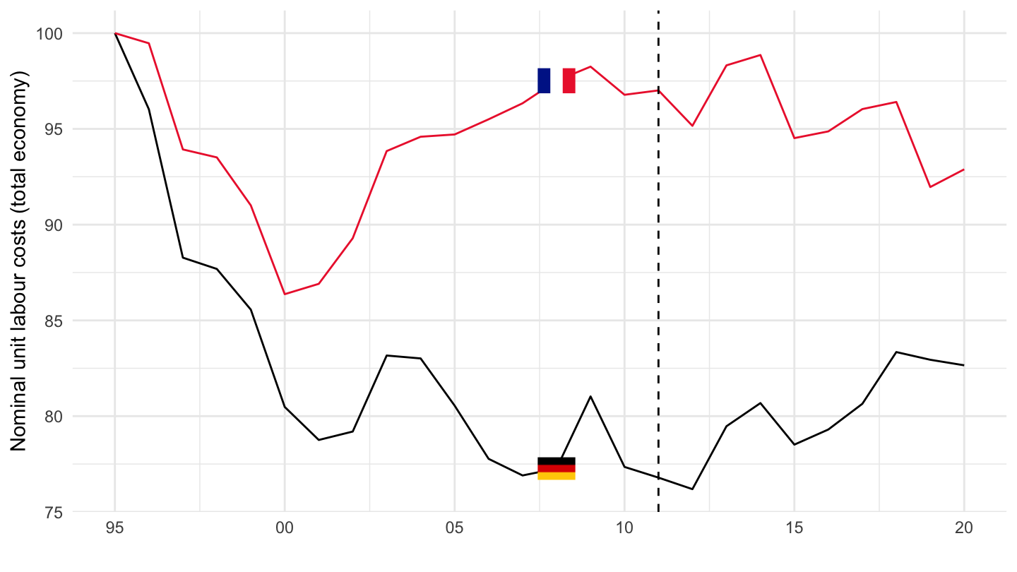
France, Germany, Spain, Italy
All
Code
ameco %>%
  filter(VAR == "PLCDQ",
         COU %in% c("FRA", "DEU", "ESP", "ITA"),
         CODE_4 == "30",
         CODE_5 == "437") %>%
  select(COUNTRY, date, value, CODE) %>%
  arrange(COUNTRY, date) %>%
  left_join(colors, c("COUNTRY" = "country")) %>%
  ggplot() + ylab("Nominal unit labour costs (total economy)") + xlab("") + theme_minimal() +
  geom_line(aes(x = date, y = value, color = color)) +
  scale_color_identity() + add_4flags +
  scale_x_date(breaks = seq(1920, 2025, 5) %>% paste0("-01-01") %>% as.Date,
               labels = date_format("%y")) +
  theme(legend.position = c(0.2, 0.8),
        legend.title = element_blank()) +
  scale_y_continuous(breaks = seq(-60, 300, 5))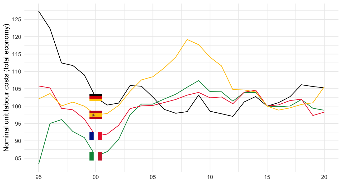
1999-
Code
ameco %>%
  filter(VAR == "PLCDQ",
         COU %in% c("FRA", "DEU", "ESP", "ITA"),
         CODE_4 == "30",
         CODE_5 == "437") %>%
  select(COUNTRY, date, value, CODE) %>%
  arrange(COUNTRY, date) %>%
  filter(date >= as.Date("2000-01-01")) %>%
  group_by(COUNTRY) %>%
  mutate(value = 100*value/value[1]) %>%
  left_join(colors, c("COUNTRY" = "country")) %>%
  ggplot() + ylab("Nominal unit labour costs (total economy)") + xlab("") + theme_minimal() +
  geom_line(aes(x = date, y = value, color = COUNTRY)) +
  scale_color_manual(values = c("#002395", "#000000", "#009246", "#C60B1E")) +
  scale_x_date(breaks = seq(1920, 2025, 5) %>% paste0("-01-01") %>% as.Date,
               labels = date_format("%y")) +
  theme(legend.position = c(0.2, 0.8),
        legend.title = element_blank()) +
  scale_y_continuous(breaks = seq(-60, 300, 5))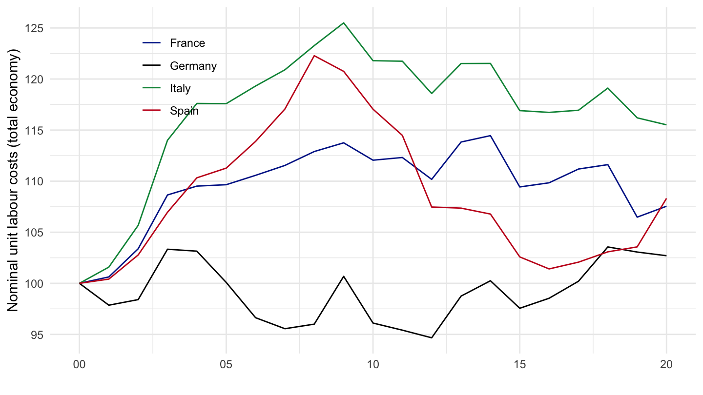
HWCMW - Nominal compensation per employee: manufacturing industry
France, Germany
All
Code
ameco %>%
  filter(VAR == "HWCMW",
         COU %in% c("FRA", "DEU"),
         CODE_4 == "99") %>%
  select(COUNTRY, date, value, CODE) %>%
  arrange(COUNTRY, date) %>%
  left_join(colors, c("COUNTRY" = "country")) %>%
  ggplot() + ylab("Nominal compensation per employee: manufacturing") + xlab("") + theme_minimal() +
  geom_line(aes(x = date, y = value, color = color)) +
  scale_color_identity() + add_2flags +
  scale_x_date(breaks = seq(1920, 2025, 5) %>% paste0("-01-01") %>% as.Date,
               labels = date_format("%y")) +
  theme(legend.position = c(0.8, 0.1),
        legend.title = element_blank()) +
  scale_y_continuous(breaks = seq(-60, 300, 5))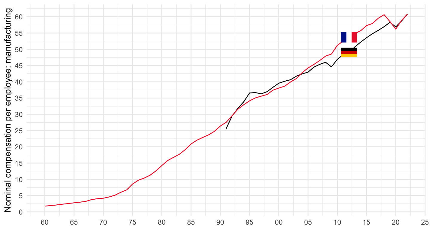
1995-
Code
ameco %>%
  filter(VAR == "HWCMW",
         COU %in% c("FRA", "DEU"),
         CODE_4 == "99",
         date >= as.Date("1995-01-01")) %>%
  select(COUNTRY, date, value, CODE) %>%
  arrange(COUNTRY, date) %>%
  left_join(colors, c("COUNTRY" = "country")) %>%
  ggplot() + ylab("Nominal compensation per employee: manufacturing") + xlab("") + theme_minimal() +
  geom_line(aes(x = date, y = value, color = color)) +
  scale_color_identity() + add_2flags +
  scale_x_date(breaks = seq(1920, 2025, 5) %>% paste0("-01-01") %>% as.Date,
               labels = date_format("%y")) +
  theme(legend.position = c(0.8, 0.1),
        legend.title = element_blank()) +
  scale_y_continuous(breaks = seq(-60, 300, 5))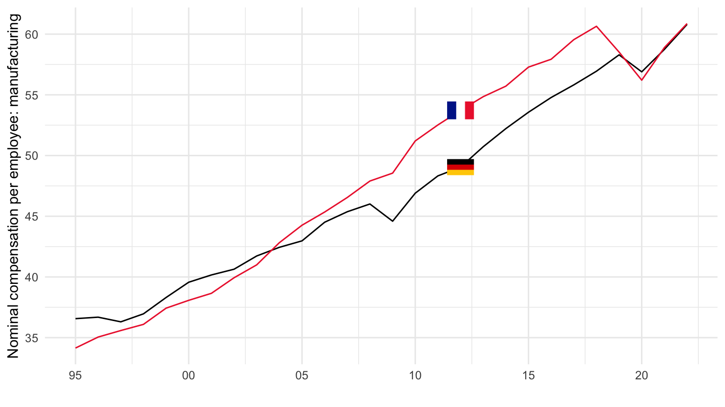
France, Germany, Spain, Italy
All
Code
ameco %>%
  filter(VAR == "HWCMW",
         COU %in% c("FRA", "DEU", "ESP", "ITA"),
         CODE_4 == "99") %>%
  select(COUNTRY, date, value, CODE) %>%
  arrange(COUNTRY, date) %>%
  group_by(COUNTRY) %>%
  mutate(value = 100*value/value[1]) %>%
  left_join(colors, c("COUNTRY" = "country")) %>%
  ggplot() + ylab("Nominal compensation per employee: manufacturing industry") + xlab("") + theme_minimal() +
  geom_line(aes(x = date, y = value, color = color)) +
  scale_color_identity() + add_4flags +
  scale_x_date(breaks = seq(1920, 2025, 5) %>% paste0("-01-01") %>% as.Date,
               labels = date_format("%y")) +
  theme(legend.position = c(0.2, 0.8),
        legend.title = element_blank()) +
  scale_y_log10(breaks = seq(-60, 300, 5))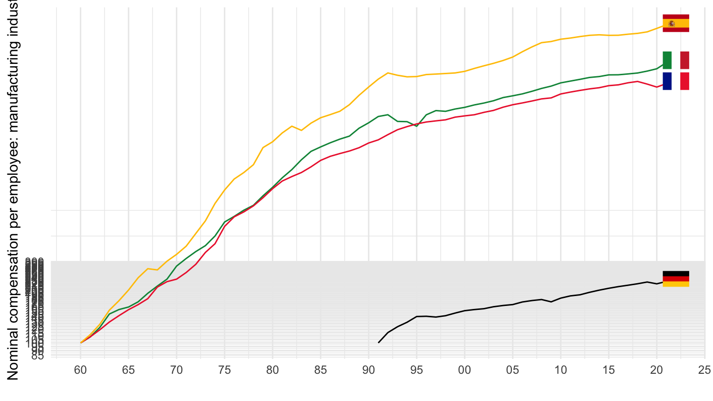
1999-
Code
ameco %>%
  filter(VAR == "HWCMW",
         COU %in% c("FRA", "DEU", "ESP", "ITA"),
         CODE_4 == "99",
         date >= as.Date("1999-01-01")) %>%
  select(COUNTRY, date, value, CODE) %>%
  arrange(COUNTRY, date) %>%
  filter(date >= as.Date("1999-01-01")) %>%
  group_by(COUNTRY) %>%
  mutate(value = 100*value/value[1]) %>%
  left_join(colors, c("COUNTRY" = "country")) %>%
  ggplot() + ylab("Nominal compensation per employee: manufacturing industry") + xlab("") + theme_minimal() +
  geom_line(aes(x = date, y = value, color = color)) +
  scale_color_identity() + add_4flags +
  scale_x_date(breaks = seq(1920, 2025, 5) %>% paste0("-01-01") %>% as.Date,
               labels = date_format("%y")) +
  theme(legend.position = c(0.2, 0.8),
        legend.title = element_blank()) +
  scale_y_log10(breaks = seq(-60, 300, 5))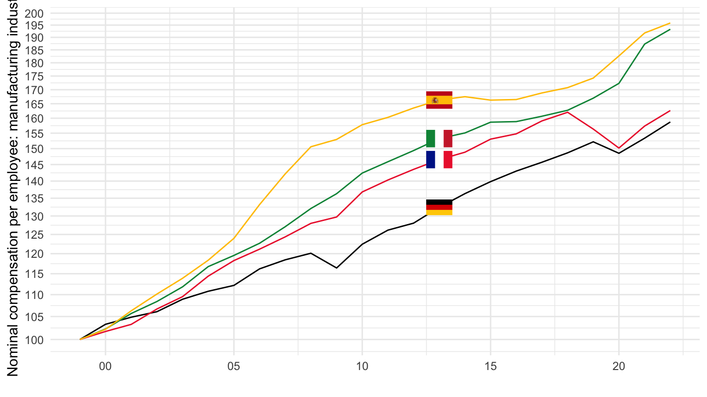
QLCM - Real unit labour costs: manufacturing industry
France, Germany
Code
ameco %>%
  filter(VAR == "QLCM",
         COU %in% c("FRA", "DEU")) %>%
  select(COUNTRY, date, value, CODE) %>%
  arrange(COUNTRY, date) %>%
  left_join(colors, c("COUNTRY" = "country")) %>%
  ggplot() + ylab("Real unit labour costs (manufacturing)") + xlab("") + theme_minimal() +
  geom_line(aes(x = date, y = value, color = color)) +
  scale_color_identity() + add_2flags +
  scale_x_date(breaks = seq(1920, 2025, 5) %>% paste0("-01-01") %>% as.Date,
               labels = date_format("%y")) +
  theme(legend.position = c(0.8, 0.1),
        legend.title = element_blank()) +
  scale_y_continuous(breaks = seq(-60, 300, 5))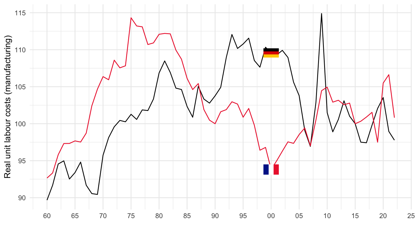
France, Germany, Spain, Italy
###All
Code
ameco %>%
  filter(VAR == "QLCM",
         COU %in% c("FRA", "DEU", "ESP", "ITA")) %>%
  select(COUNTRY, date, value, CODE) %>%
  arrange(COUNTRY, date) %>%
  left_join(colors, c("COUNTRY" = "country")) %>%
  ggplot() + ylab("Real unit labour costs (manufacturing)") + xlab("") + theme_minimal() +
  geom_line(aes(x = date, y = value, color = color)) +
  scale_color_identity() + add_4flags +
  scale_x_date(breaks = seq(1920, 2025, 5) %>% paste0("-01-01") %>% as.Date,
               labels = date_format("%y")) +
  theme(legend.position = c(0.2, 0.8),
        legend.title = element_blank()) +
  scale_y_continuous(breaks = seq(-60, 300, 5))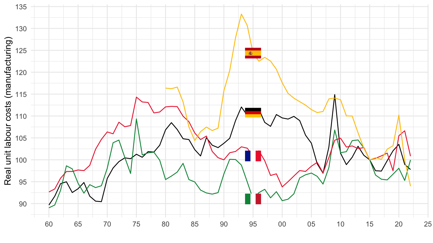
1999-
Code
ameco %>%
  filter(VAR == "QLCM",
         COU %in% c("FRA", "DEU", "ESP", "ITA")) %>%
  select(COUNTRY, date, value, CODE) %>%
  arrange(COUNTRY, date) %>%
  filter(date >= as.Date("1999-01-01")) %>%
  group_by(COUNTRY) %>%
  mutate(value = 100*value/value[1]) %>%
  left_join(colors, c("COUNTRY" = "country")) %>%
  ggplot() + ylab("Real unit labour costs (manufacturing)") + xlab("") + theme_minimal() +
  geom_line(aes(x = date, y = value, color = color)) +
  scale_color_identity() + add_4flags +
  scale_x_date(breaks = seq(1999, 2025, 2) %>% paste0("-01-01") %>% as.Date,
               labels = date_format("%Y")) +
  theme(legend.position = c(0.2, 0.8),
        legend.title = element_blank()) +
  scale_y_continuous(breaks = seq(-60, 300, 5))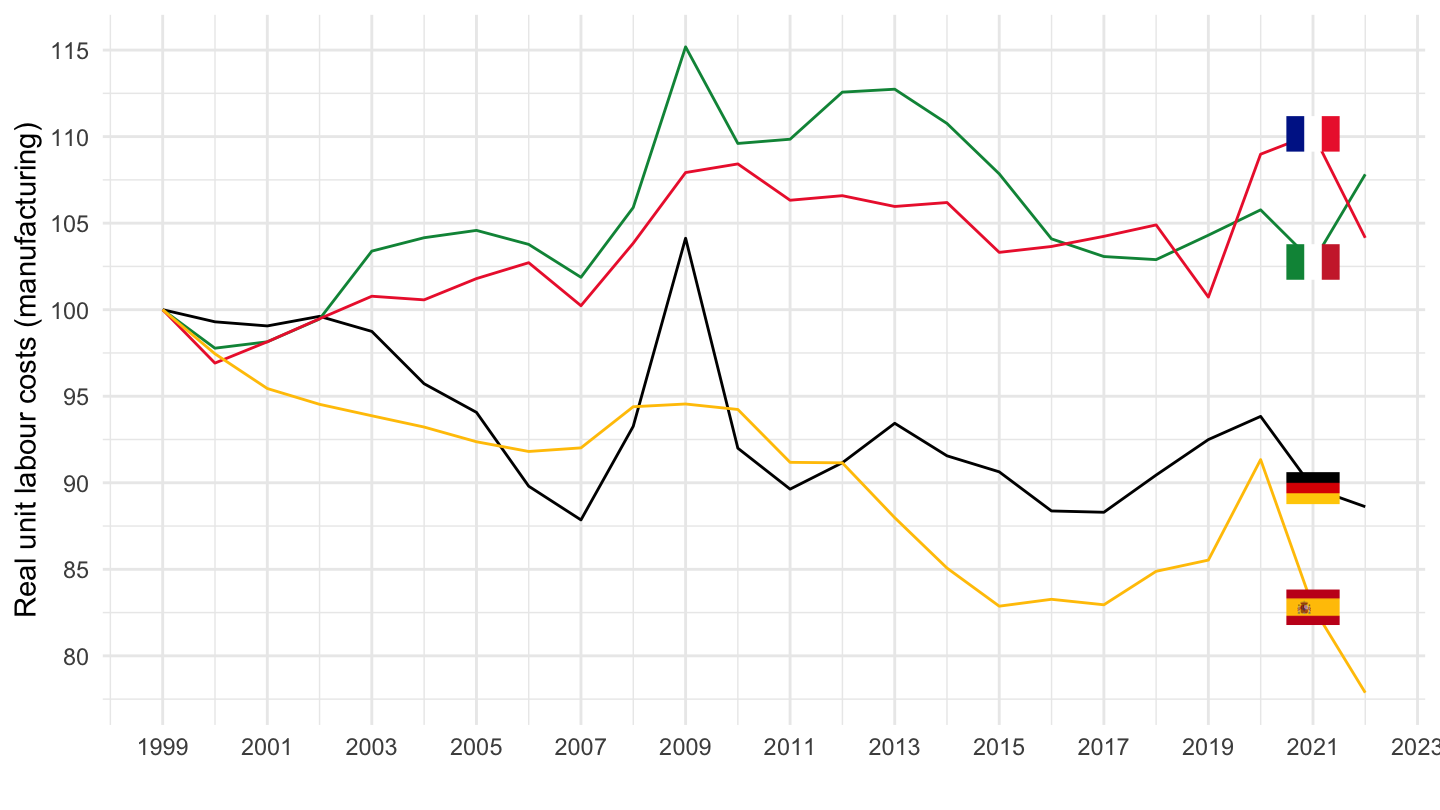
PLCM - Nominal unit labour costs: manufacturing industry
France, Germany
All
Code
ameco %>%
  filter(VAR == "PLCM",
         COU %in% c("FRA", "DEU"),
         CODE_4 == "99") %>%
  select(COUNTRY, date, value, CODE) %>%
  arrange(COUNTRY, date) %>%
  left_join(colors, c("COUNTRY" = "country")) %>%
  ggplot() + ylab("Nominal unit labour costs (manufacturing)") + xlab("") + theme_minimal() +
  geom_line(aes(x = date, y = value, color = color)) +
  scale_color_identity() + add_2flags +
  scale_x_date(breaks = seq(1920, 2025, 5) %>% paste0("-01-01") %>% as.Date,
               labels = date_format("%y")) +
  theme(legend.position = c(0.2, 0.9),
        legend.title = element_blank()) +
  scale_y_continuous(breaks = seq(-60, 300, 10))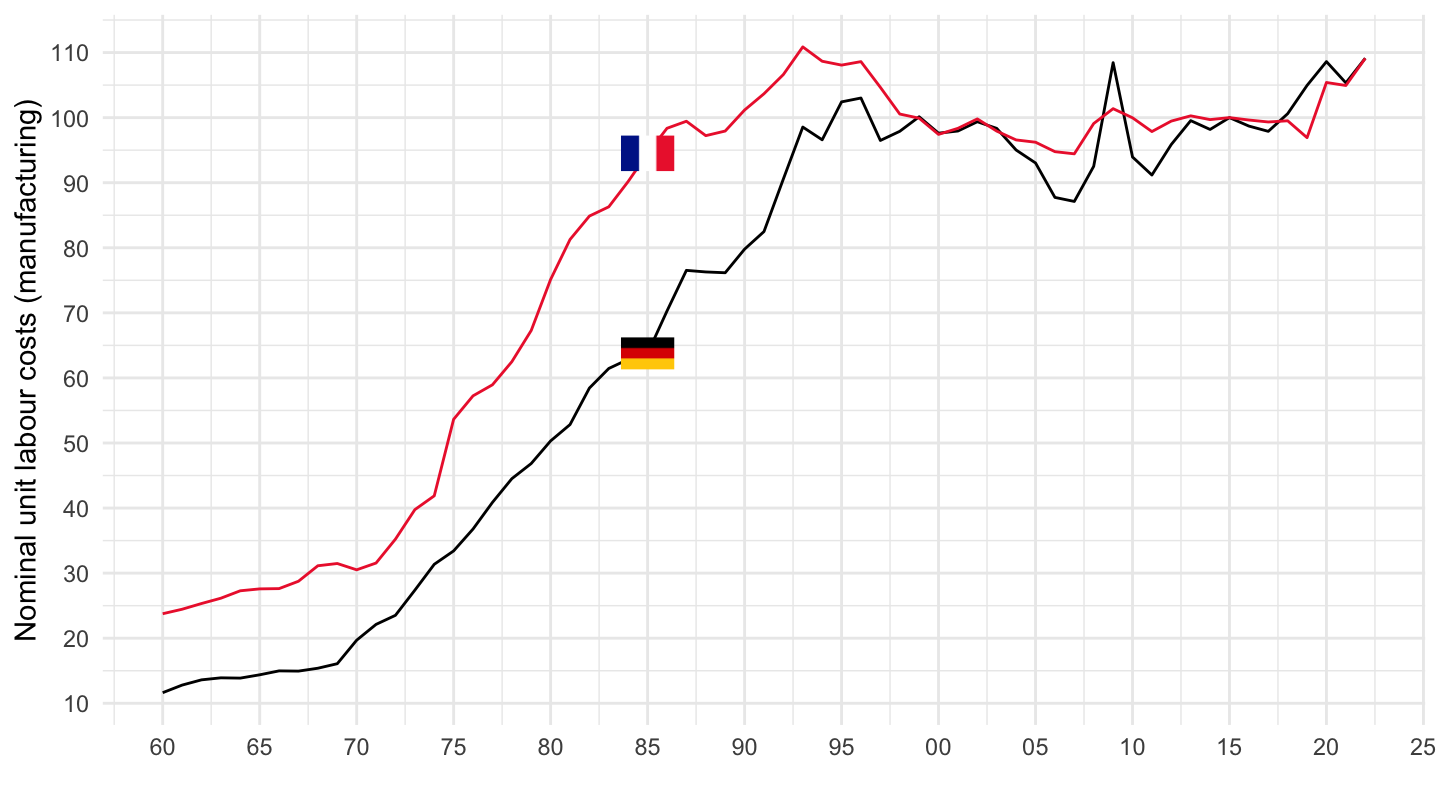
1990-
Code
ameco %>%
  filter(VAR == "PLCM",
         COU %in% c("FRA", "DEU"),
         CODE_4 == "99") %>%
  select(COUNTRY, date, value, CODE) %>%
  arrange(COUNTRY, date) %>%
  left_join(colors, c("COUNTRY" = "country")) %>%
  filter(date >= as.Date("1990-01-01")) %>%
  ggplot() + ylab("Nominal unit labour costs (manufacturing)") + xlab("") + theme_minimal() +
  geom_line(aes(x = date, y = value, color = color)) +
  scale_color_identity() + add_2flags +
  scale_x_date(breaks = seq(1920, 2025, 2) %>% paste0("-01-01") %>% as.Date,
               labels = date_format("%y")) +
  theme(legend.position = c(0.8, 0.2),
        legend.title = element_blank()) +
  scale_y_continuous(breaks = seq(-60, 300, 10))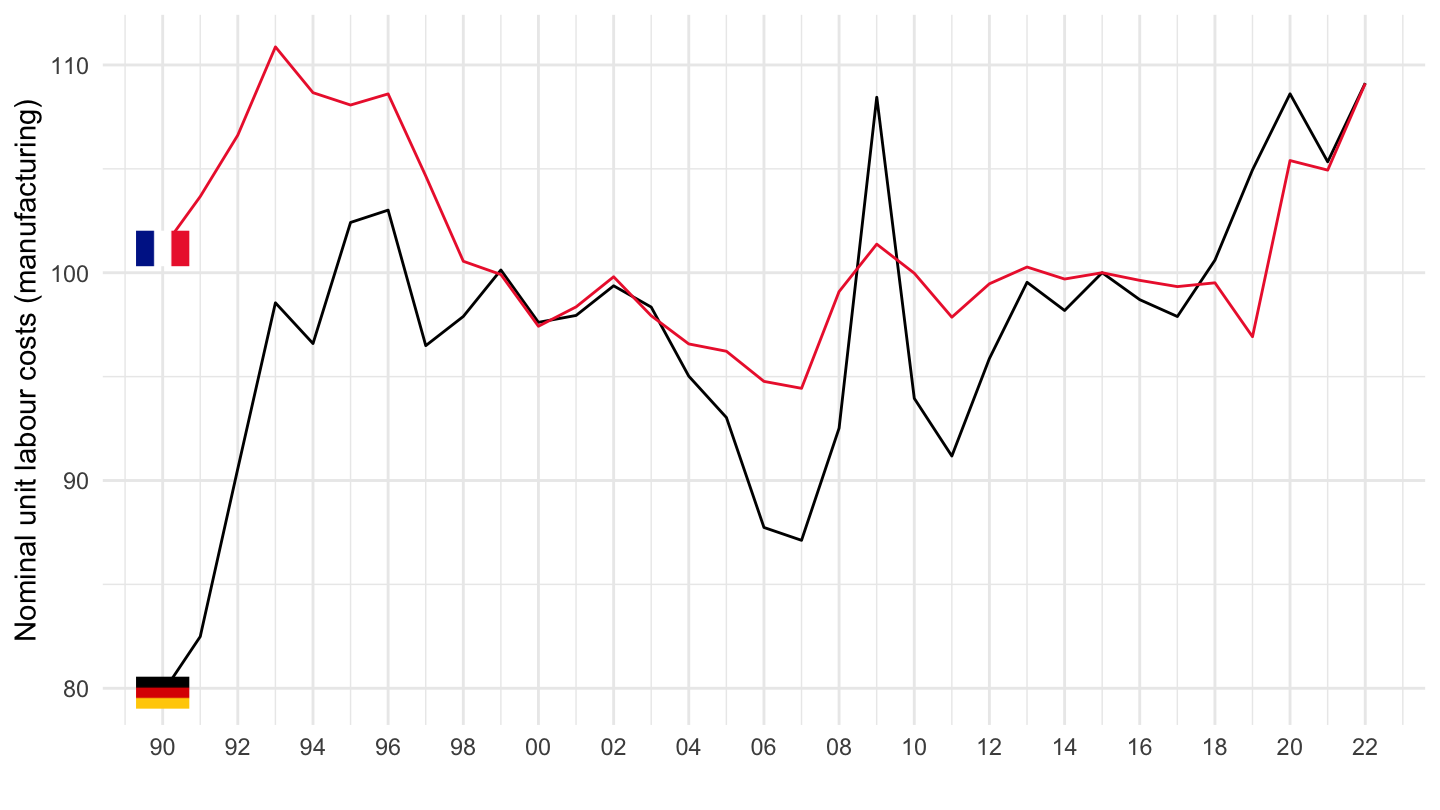
France, Germany, Spain, Italy
All
Code
ameco %>%
  filter(VAR == "PLCM",
         COU %in% c("FRA", "DEU", "ESP", "ITA"),
         CODE_4 == "99") %>%
  select(COUNTRY, date, value, CODE) %>%
  arrange(COUNTRY, date) %>%
  left_join(colors, c("COUNTRY" = "country")) %>%
  ggplot() + ylab("Nominal unit labour costs (manufacturing)") + xlab("") + theme_minimal() +
  geom_line(aes(x = date, y = value, color = color)) +
  scale_color_identity() + add_4flags +
  scale_x_date(breaks = seq(1920, 2025, 5) %>% paste0("-01-01") %>% as.Date,
               labels = date_format("%y")) +
  theme(legend.position = c(0.2, 0.8),
        legend.title = element_blank()) +
  scale_y_continuous(breaks = seq(-60, 300, 5))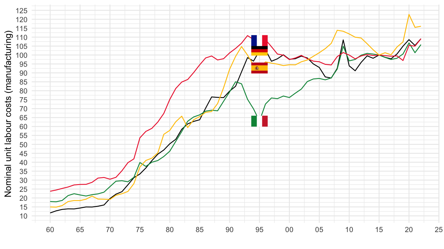
1999-
Code
ameco %>%
  filter(VAR == "PLCM",
         COU %in% c("FRA", "DEU", "ESP", "ITA"),
         CODE_4 == "99") %>%
  select(COUNTRY, date, value, CODE) %>%
  arrange(COUNTRY, date) %>%
  filter(date >= as.Date("1999-01-01")) %>%
  group_by(COUNTRY) %>%
  mutate(value = 100*value/value[1]) %>%
  left_join(colors, c("COUNTRY" = "country")) %>%
  ggplot() + ylab("Coûts unitaires du travail, nominal (secteur manuf.)") + xlab("") + theme_minimal() +
  geom_line(aes(x = date, y = value, color = color)) +
  scale_color_identity() +
  scale_x_date(breaks = seq(1999, 2023, 2) %>% paste0("-01-01") %>% as.Date,
               labels = date_format("%Y")) +
  add_4flags +
  theme(legend.position = c(0.2, 0.8),
        legend.title = element_blank()) +
  scale_y_continuous(breaks = seq(-60, 300, 5))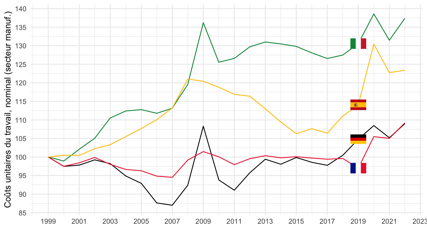
1995-
Viridis Colors
Code
ameco %>%
  filter(VAR == "PLCM",
         COU %in% c("FRA", "DEU", "ESP", "ITA"),
         CODE_4 == "99") %>%
  select(COUNTRY, date, value, CODE) %>%
  arrange(COUNTRY, date) %>%
  filter(date >= as.Date("1995-01-01")) %>%
  group_by(COUNTRY) %>%
  mutate(value = 100*value/value[1]) %>%
  left_join(colors, c("COUNTRY" = "country")) %>%
  ggplot() + ylab("Nominal unit labour costs (manufacturing)") + xlab("") + theme_minimal() +
  geom_line(aes(x = date, y = value, color = color)) +
  scale_color_identity() + add_4flags +
  scale_x_date(breaks = seq(1920, 2025, 2) %>% paste0("-01-01") %>% as.Date,
               labels = date_format("%y")) +
  geom_vline(xintercept = as.Date("2011-01-01"),
             linetype= "dashed") +
  theme(legend.position = c(0.2, 0.8),
        legend.title = element_blank()) +
  scale_y_continuous(breaks = seq(-60, 300, 5))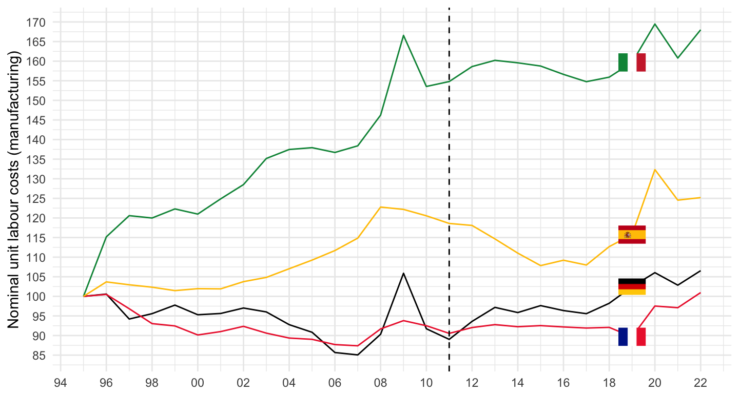
PLCD - Nominal unit labour costs: total economy (Ratio of compensation per employee to real GDP per person employed.)
France, Germany
All
Code
ameco %>%
  filter(VAR == "PLCD",
         COU %in% c("FRA", "DEU"),
         CODE_4 == "99") %>%
  select(COUNTRY, date, value, CODE) %>%
  arrange(COUNTRY, date) %>%
  left_join(colors, c("COUNTRY" = "country")) %>%
  ggplot() + ylab("Nominal unit labour costs") + xlab("") + theme_minimal() +
  geom_line(aes(x = date, y = value, color = color)) +
  scale_color_identity() + add_2flags +
  scale_x_date(breaks = seq(1920, 2025, 5) %>% paste0("-01-01") %>% as.Date,
               labels = date_format("%y")) +
  theme(legend.position = c(0.2, 0.9),
        legend.title = element_blank()) +
  scale_y_continuous(breaks = seq(-60, 300, 10))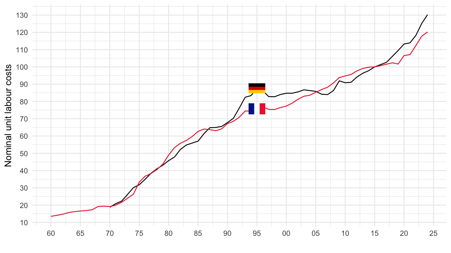
1995-
Viridis Colors
Code
ameco %>%
  filter(VAR == "PLCD",
         COU %in% c("FRA", "DEU"),
         CODE_4 == "99") %>%
  select(COUNTRY, date, value, CODE) %>%
  filter(date >= as.Date("1995-01-01"),
         date <= as.Date("2020-01-01")) %>%
  group_by(COUNTRY) %>%
  mutate(value = 100*value/value[date == as.Date("1995-01-01")]) %>%
  arrange(COUNTRY, date) %>%
  left_join(colors, c("COUNTRY" = "country")) %>%
  ggplot() + ylab("Nominal unit labour costs") + xlab("") + theme_minimal() +
  geom_line(aes(x = date, y = value, color = color)) +
  scale_color_identity() + add_2flags +
  scale_x_date(breaks = seq(1920, 2025, 5) %>% paste0("-01-01") %>% as.Date,
               labels = date_format("%Y")) +
  theme(legend.position = c(0.2, 0.9),
        legend.title = element_blank()) +
  scale_y_log10(breaks = seq(-60, 300, 10))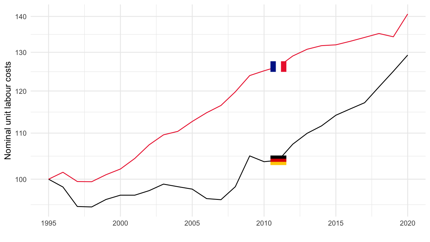
1999-
Viridis Colors
Code
ameco %>%
  filter(VAR == "PLCD",
         COU %in% c("FRA", "DEU"),
         CODE_4 == "99") %>%
  select(COUNTRY, date, value, CODE) %>%
  filter(date >= as.Date("1999-01-01")) %>%
  group_by(COUNTRY) %>%
  mutate(value = 100*value/value[date == as.Date("1999-01-01")]) %>%
  arrange(COUNTRY, date) %>%
  left_join(colors, c("COUNTRY" = "country")) %>%
  ggplot() + ylab("Nominal unit labour costs") + xlab("") + theme_minimal() +
  geom_line(aes(x = date, y = value, color = color)) +
  scale_color_identity() + add_2flags +
  scale_x_date(breaks = seq(1920, 2025, 2) %>% paste0("-01-01") %>% as.Date,
               labels = date_format("%y")) +
  theme(legend.position = c(0.2, 0.9),
        legend.title = element_blank()) +
  scale_y_log10(breaks = seq(-60, 300, 10))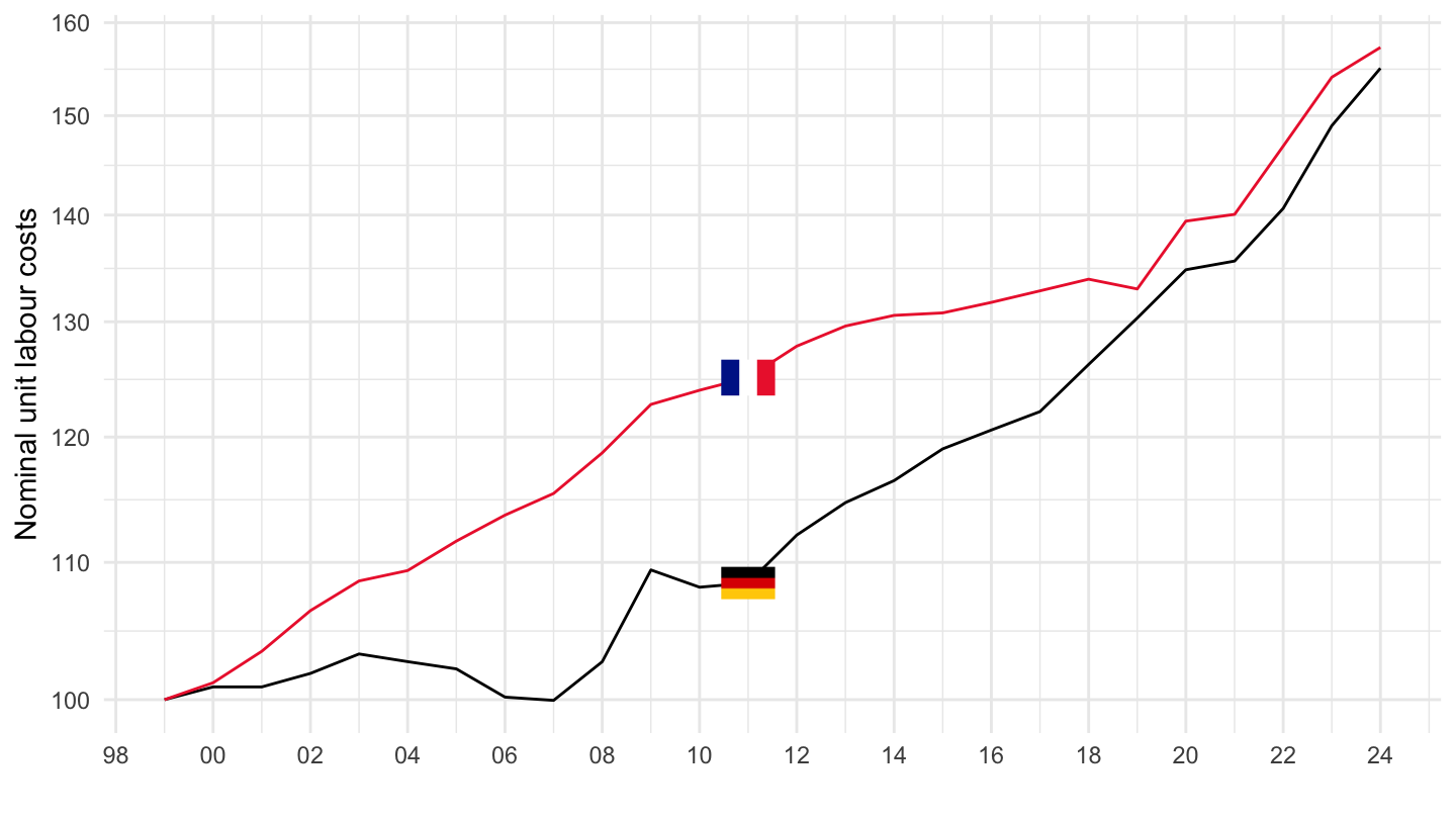
Flags
Code
ameco %>%
  filter(VAR == "PLCD",
         COU %in% c("FRA", "DEU", "ITA"),
         CODE_4 == "99") %>%
  select(COUNTRY, date, value, CODE) %>%
  filter(date >= as.Date("1995-01-01"),
         date <= as.Date("2020-01-01")) %>%
  group_by(COUNTRY) %>%
  mutate(value = 100*value/value[date == as.Date("1995-01-01")]) %>%
  arrange(COUNTRY, date) %>%
  left_join(colors, c("COUNTRY" = "country")) %>%
  ggplot() + ylab("Coûts Unitaires du Travail (Source: AMECO)") + xlab("") + theme_minimal() +
  geom_line(aes(x = date, y = value, color = color)) +
  scale_color_identity() + add_3flags +
  scale_x_date(breaks = seq(1920, 2025, 2) %>% paste0("-01-01") %>% as.Date,
               labels = date_format("%y")) +
  theme(legend.position = "none") +
  scale_y_log10(breaks = seq(-60, 300, 10))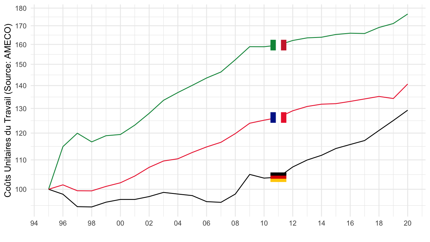
France, Germany, Spain, Italy
All
Code
ameco %>%
  filter(VAR == "PLCD",
         COU %in% c("FRA", "DEU", "ESP", "ITA"),
         CODE_4 == "99") %>%
  select(COUNTRY, date, value, CODE) %>%
  arrange(COUNTRY, date) %>%
  left_join(colors, c("COUNTRY" = "country")) %>%
  ggplot() + ylab("Nominal unit labour costs (total economy)") + xlab("") + theme_minimal() +
  geom_line(aes(x = date, y = value, color = color)) +
  scale_color_identity() + add_4flags +
  scale_x_date(breaks = seq(1920, 2025, 5) %>% paste0("-01-01") %>% as.Date,
               labels = date_format("%y")) +
  theme(legend.position = c(0.2, 0.8),
        legend.title = element_blank()) +
  scale_y_continuous(breaks = seq(-60, 300, 5))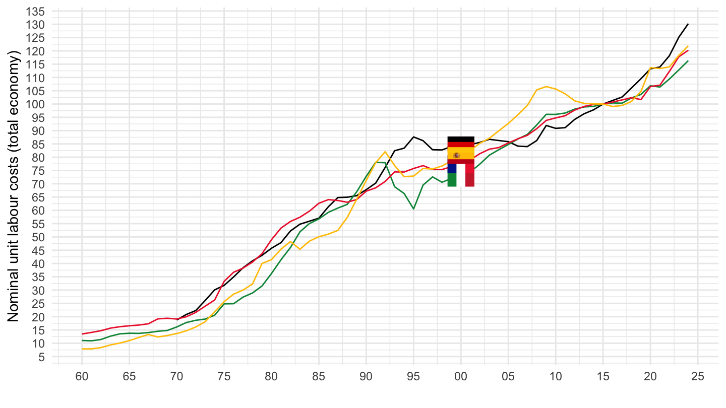
1999-
Code
ameco %>%
  filter(VAR == "PLCD",
         COU %in% c("FRA", "DEU", "ESP", "ITA"),
         CODE_4 == "99") %>%
  select(COUNTRY, date, value, CODE) %>%
  arrange(COUNTRY, date) %>%
  filter(date >= as.Date("1999-01-01")) %>%
  group_by(COUNTRY) %>%
  mutate(value = 100*value/value[1]) %>%
  left_join(colors, c("COUNTRY" = "country")) %>%
  ggplot() + ylab("Coûts unitaires du travail, nominal (total)") + xlab("") + theme_minimal() +
  geom_line(aes(x = date, y = value, color = color)) +
  scale_color_identity() + add_4flags +
  scale_x_date(breaks = seq(1901, 2025, 2) %>% paste0("-01-01") %>% as.Date,
               labels = date_format("%Y")) +
  add_4flags +
  theme(legend.position = c(0.2, 0.8),
        legend.title = element_blank()) +
  scale_y_continuous(breaks = seq(-60, 300, 5))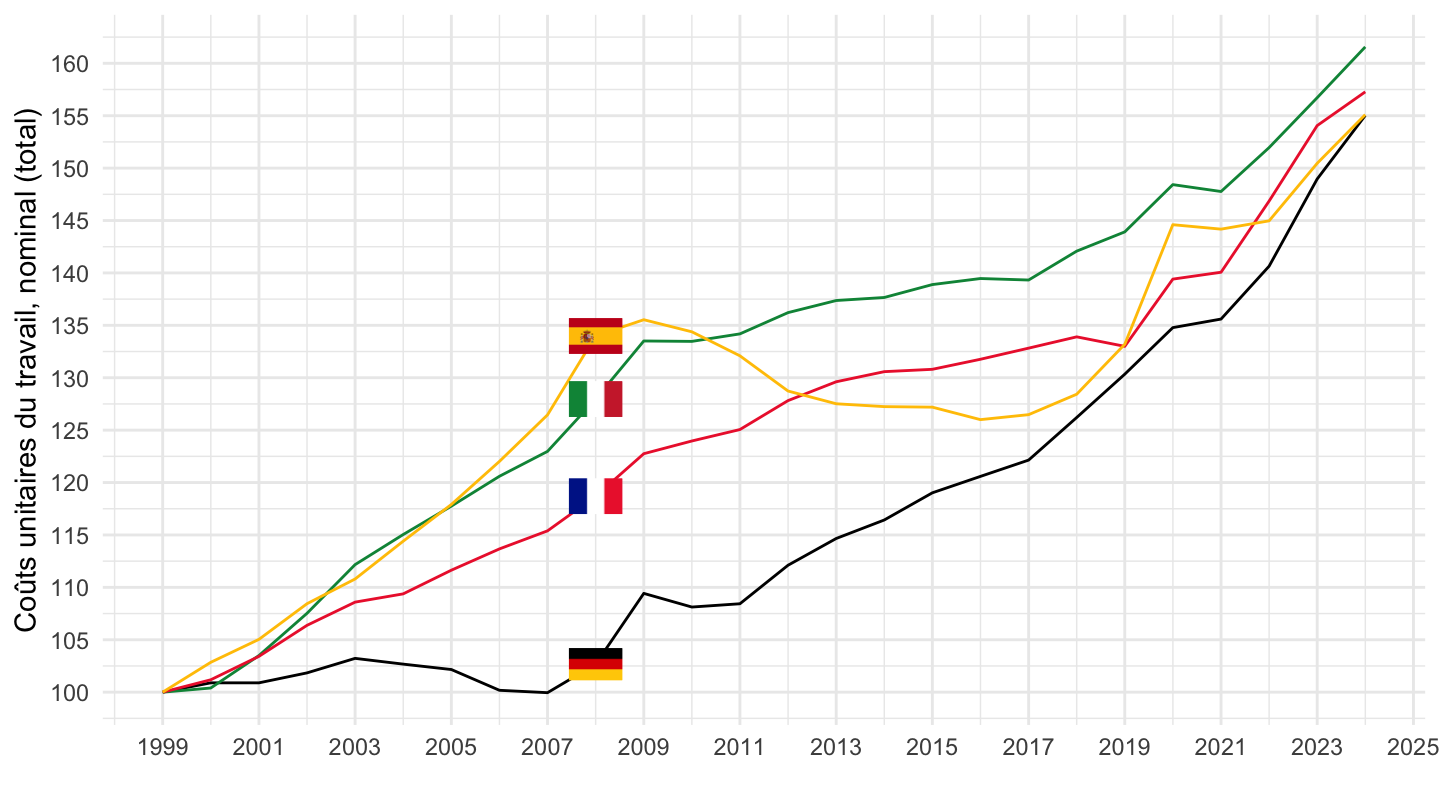
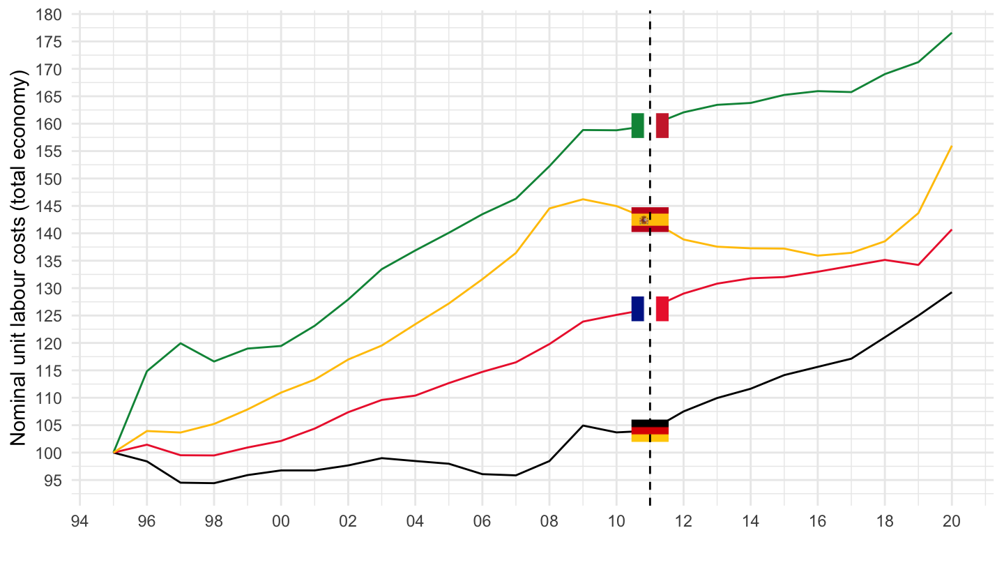
1995-
Code
ameco %>%
  filter(VAR == "PLCD",
         COU %in% c("FRA", "DEU", "ESP", "ITA"),
         CODE_4 == "99") %>%
  select(COUNTRY, date, value, CODE) %>%
  arrange(COUNTRY, date) %>%
  filter(date >= as.Date("1995-01-01"),
         date <= as.Date("2020-01-01")) %>%
  group_by(COUNTRY) %>%
  mutate(value = 100*value/value[1]) %>%
  left_join(colors, c("COUNTRY" = "country")) %>%
  ggplot() + ylab("Nominal unit labour costs (total economy)") + xlab("") + theme_minimal() +
  geom_line(aes(x = date, y = value, color = color)) +
  scale_color_identity() + add_4flags +
  scale_x_date(breaks = seq(1920, 2025, 2) %>% paste0("-01-01") %>% as.Date,
               labels = date_format("%y")) +
  geom_vline(xintercept = as.Date("2011-01-01"),
             linetype= "dashed") +
  theme(legend.position = c(0.2, 0.8),
        legend.title = element_blank()) +
  scale_y_continuous(breaks = seq(-60, 300, 5))