Reassessing Dynamic Efficiency2
François Geerolf1
Abstract
Keywords: Dynamic efficiency, savings glut, marginal returns to capital.
JEL classification: E21, E22, E24.
Introduction
Caselli and Feyrer (2007)
Since the neoclassical synthesis, it is usually believed that
I also show that average returns are a very poor way of measuring the marginal returns to capital, as they are very different objects in theor. I first develop some theory which shows that the marginal returns to capital can actually be equal to zero, and yet,
I then interpret Romer and Romer (2010) evidence as a shock to public saving, which according to neoclassical theory should reduce the interest rate and boost investment. Empirically, this is not what jappens - in fgact, investment falls following an increase in public saving.
I then distingish between the expected and realized returns to capital. I argue that the large returns experienced post World War II on the U.S. stock market, and the large returns experienced on real estate assets in many other countries, were not expected and cannot therefore be seen as the marginal return to capital. Another way to say this is that the marginal project which was undertaken during this period was in fact much lower, closer to the risk free rate.
Although the difference in returns between equity and houses and government debt is usually attributed to riskiness, I in contrast connect it to the infinitely lived nature of these assets, which implies that they can carry a “rational bubble”. Assuming dynamic inefficiency, these rational bubbles are indeed feasible. (Tirole (1985))
I also show that the average return to capital, as measured by the capital share divided by the stock of capital, leads to greatly overstate the marginal return to capital. The reasons are multiple
Finally,
Moreover,
Dynamic efficiency is an important macroeconomic issue. The presumption that increasing saving is always good for the economy relies on the fact that more saving implies more investment adding to the capital stock, that a higher capital stock leads to more output in the long run, and that more output ultimately helps achieve higher consumption. The first fact is mechanical, But the second is not necessarily true, because more capital also means more investment to maintain the same capital/output ratio. Consequently, there are limits as to how much capital should ideally be accumulated. According to the neoclassical theory, the amount of capital such that the flow of consumption is maximized is called the Golden Rule level of capital, which is reached when the interest rate r is equal to the rate of growth of the economy g (Ramsey (1928), Phelps (1961), Phelps (1965), Diamond (1965)). If the capital stock installed is higher than the Golden Rule or r<g, then every agent could be made better off by consuming the capital so that the Golden-Rule level is restored.Note that according to a steady-state welfare criterion, capital underaccumulation (with r>g) is also suboptimal. However the transitional dynamics to this new steady state are costly for the generations who therefore need to consume less and accumulate capital. A competitive equilibrium with optimizing agents, market clearing and price taking can lead to such a situation of over-accumulation, even without assuming any type of inefficiency. All that is needed is that the economy is expected to run forever.
Discussions between
1 Capital and the Production Function
1.1 Much capital is not
The Solow (1956) growth model

Figure 1.1: Dynamic Efficiency, Dynamic Inefficiency, Secular Stagnation
2 What is capital?
2.1 Costs of waiting
2.2 Not entrepreneutrial labor
As Piketty (2014) says: “Bear in mind, too, that a portion of what is called the income of capital may be remuneration for entrepreneurial labor, and this should no doubt be treated as we treat other forms of labor. This classic argument deserves closer scrutiny”
2.3 Rational Bubbles
Tirole (1985)
3 Aggregate Time Series
3.1 Business Cycle Evidence
3.2 (???)
To the extent that tax increases lead to an increase in public saving, they lead to a paradox of thrift:
If investment is not interest elastic, and the interest elasticity is equal to zero, then there should be no change in investment coming from the change in the cost of capital.
3.3 Event Studies: Pension Reform
Movements from a pay-as-you-go system to a funded syetem, pushed in particular by the Organization for Economic Development (OECD) lead to an increase in the aggregate saving rate. In 2001, then Chancellor of Germany Gerhard Schröder reformed the German Pension system.
4 Macroeconomic Evidence
4.1 Riester Reforms in Germany (2001)
4.2 Pension reform in Spain (2005)
4.3 Does more saving lead to more investment?
Recessions are times where saving increases
4.4 Examples to understand better what capital is
Say that the government were to tax land at some rate, and promise that future land would be taxed.
More generally, future capital taxation destroys stores of values, which implies that there arre actually not enugh stores of value.
In the secular stagnation regime, this leads to dynamic inefficiency potentially, and it potentially helps capital accumulation. Maybe we have too high capital income taxation, which implies that future taxes are not taxed the way that they should. De facto real estate bubbles are not taxed because ineheritances are not taxed. As a consequence,
4.5
5 Cross-sectional Evidence
Do Apple profits correspond to much accumulated capital? The answer is clearly, no.
How do you explain the profits from the financial industry? Does it have anything to do with capital-labor substitution? Rognlie (2015)
6 What is substitutable with labor?
Is IPP capital really substitutable with labor?
In macroeconomics textbook “capital” is said to be substitutable with labor. However are structures really substitutable with labor? Is it not mostly machines that are substitutable with labor?
Howeve
| Country | Buildings other than dwellings | Cultivated biological resources | Dwellings | Intellectual property product | Inventories | Machinery and equipment and weapon system |
|---|---|---|---|---|---|---|
| Australia | 147.3% | 1.4% | 112.6% | 13.6% | 10.1% | 37.7% |
| Austria | 189.7% | 0.4% | 138.8% | 19.8% | 49.2% | |
| Belgium | 88.4% | 0% | 136% | 15.6% | 19% | 50.5% |
| Canada | 88.5% | 118.8% | 11.4% | 14.7% | 20% | |
| Czech Republic | 205.1% | 0.3% | 106.2% | 11.6% | 48.1% | 69.1% |
| Denmark | 105.4% | 0.4% | 141.2% | 23.9% | 44.5% | |
| Estonia | 136.4% | 0.4% | 94.7% | 7% | 26.4% | 53.2% |
| Finland | 120.1% | 0.1% | 143.3% | 17.5% | 39.8% | 37.5% |
| France | 88.1% | 1.1% | 197.1% | 17.5% | 18.4% | 28.9% |
| Germany | 102.1% | 0.3% | 156.8% | 16.4% | 40.9% | |
| Greece | 96% | 0.3% | 157.1% | 5.4% | 26.2% | 59.9% |
| Hungary | 207.4% | 0.9% | 99.9% | 9.9% | 28% | 63.3% |
| Israel | 60.1% | 0.7% | 96.1% | 17.8% | 10.8% | 26.7% |
| Italy | 123.3% | 0.4% | 165.8% | 10.6% | 21.8% | 41.4% |
| Japan | ||||||
| Korea | 183.1% | 0.8% | 79.9% | 19.9% | 21.1% | 43.3% |
| Lithuania | 157.6% | 0.4% | 74.6% | 7.4% | 24.6% | 41.9% |
| Luxembourg | 114.6% | 0.1% | 57.2% | 5.7% | 43.8% | |
| Mexico | 115.8% | 1.4% | 121.9% | 3% | 20.2% | 123.7% |
| Netherlands | 106.8% | 0.3% | 120.6% | 20.4% | 13.5% | 42.4% |
| New Zealand | 102.5% | 0% | 128.1% | 12% | 0% | 32% |
| Portugal | 167.6% | 4.1% | 142.9% | 7.3% | 35% | 16.7% |
| Slovak Republic | 241.5% | 9.9% | 95.7% | 5.5% | 21.6% | 80.9% |
| Slovenia | 161.9% | 1.2% | 106.5% | 10.8% | 23.2% | 45% |
| Sweden | 118.4% | 1.7% | 123.7% | 25.4% | 38.5% | 50.2% |
| United Kingdom | 87.8% | 0.4% | 90.4% | 8.9% | 15.5% | 41.8% |
| United States | 133.6% | 0% | 110.1% | 22.3% | 13.7% | 40.1% |
| Type of Fixed Asset | France (% of GDP) | United States (% of GDP) |
|---|---|---|
| Buildings other than dwellings | 88.1% | 133.6% |
| Computer software and database | 6.8% | 3.8% |
| Cultivated biological resources | 1.1% | 0% |
| Dwellings | 197.1% | 110.1% |
| Entertainment, literary or artistic originals | 0.2% | 2.6% |
| Fixed assets | 332.6% | 306% |
| Fixed assets and inventories | 351% | 306% |
| Gross domestic product (expenditure approach) | 100% | 100% |
| Intellectual property product | 17.5% | 22.3% |
| Inventories | 18.4% | 13.7% |
| Machinery and equipment and weapon system | 28.9% | 40.1% |
| Mineral exploration and evaluation | 0% | 0% |
| Non-residential buildings | 33.8% | 94.6% |
| Other Intellectual property product | 0% | 0% |
| Other structures | 54.4% | 39% |
| Produced assets | 357% | 319.7% |
| Research and development | 10.5% | 15.9% |
| Tangible fixed assets | 315.1% | 283.7% |
When one thinks about capital and labor substitution
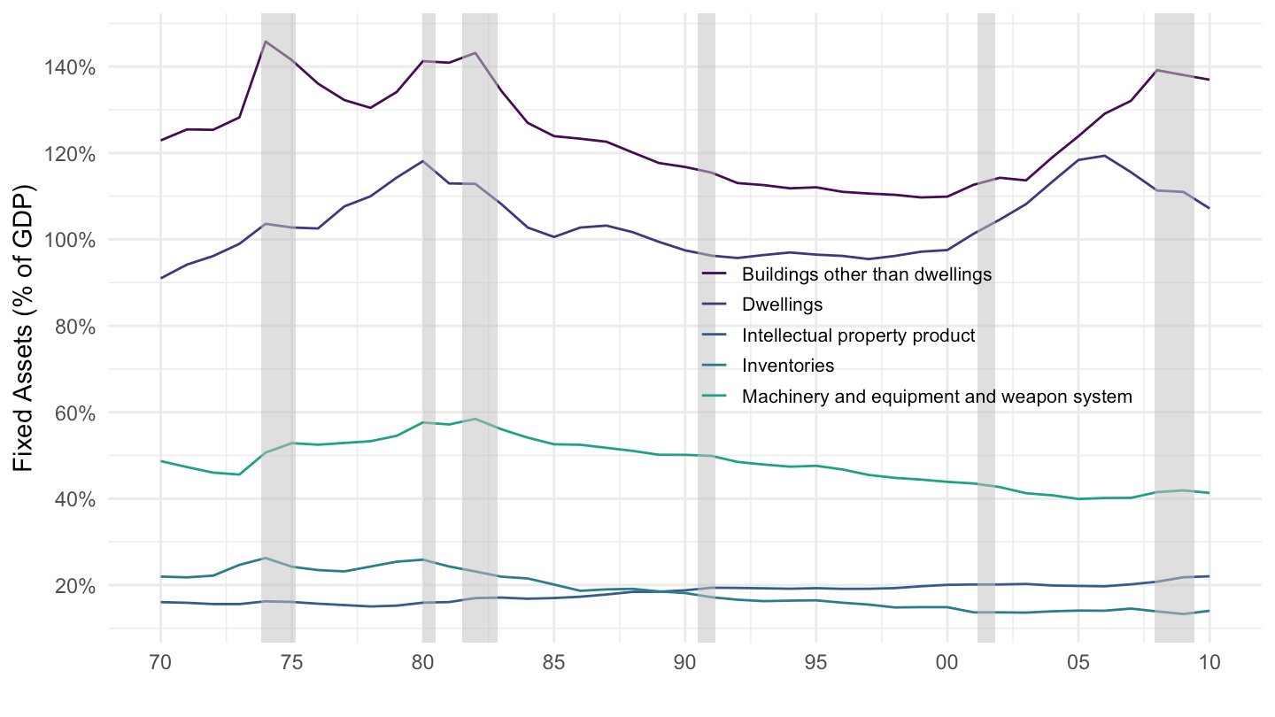
Figure 6.1: U.S. Fixed Assets (Source: OECD)

Figure 6.2: France Fixed Assets (Source: OECD)
The question is whether th
Conclusion
Moreover, market returns are superior to “preferences” for evaluating long run discount rates, unlike in Giglio, Maggiori, and Stroebel (2015).
Cochrane (2017): “But still, general equilibrium poses the central puzzle of macroeconomics since Keynes: If people want to save more, why do prices not adjust somehow so that investment is larger?”
“Corporate investment has very little relationship with real interest rates, despite the preva- lence of this channel in macroeconomic models.”
References
Abel, Andrew B., N. Gregory Mankiw, Lawrence H. Summers, and Richard J. Zeckhauser. 1989. “Assessing Dynamic Efficiency: Theory and Evidence.” The Review of Economic Studies 56 (1): 1–19. https://doi.org/10.2307/2297746.
Caselli, Francesco, and James Feyrer. 2007. “The Marginal Product of Capital.” The Quarterly Journal of Economics 122 (2): 535–68. https://doi.org/10.1162/qjec.122.2.535.
Cochrane, John H. 2017. “Macro-Finance.” Review of Finance 21 (3): 945–85. https://doi.org/10.1093/rof/rfx010.
Giglio, Stefano, Matteo Maggiori, and Johannes Stroebel. 2015. “Very Long-Run Discount Rates.” The Quarterly Journal of Economics 130 (1): 1–53. https://doi.org/10.1093/qje/qju036.
Piketty, Thomas. 2014. Capital in the Twenty-First Century. Harvard University Press.
Rognlie, Matthew. 2015. “Deciphering the Fall and Rise in the Net Capital Share: Accumulation or Scarcity?” Brookings Papers on Economic Activity, 1–54. https://www.jstor.org/stable/43684097.
Romer, Christina D., and David H. Romer. 2004. “A New Measure of Monetary Shocks: Derivation and Implications.” American Economic Review 94 (4): 1055–84. https://doi.org/10.1257/0002828042002651.
———. 2010. “The Macroeconomic Effects of Tax Changes: Estimates Based on a New Measure of Fiscal Shocks.” American Economic Review 100 (3): 763–801. https://doi.org/10.1257/aer.100.3.763.
Solow, Robert M. 1956. “A Contribution to the Theory of Economic Growth.” The Quarterly Journal of Economics 70 (1): 65–94. https://doi.org/10.2307/1884513.
Tirole, Jean. 1985. “Asset Bubbles and Overlapping Generations.” Econometrica 53 (5): 1071–1100. https://doi.org/10.2307/1911012.
Appendix
A Proofs
B Figures
B.1 Government Debt

Figure B.1: Japan’s Government Debt (Source: IMF).

Figure B.2: U.S. Government Debt (Source: IMF).
B.2 Capital
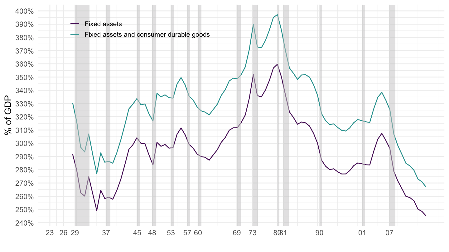
Figure B.3: Total Fixed Assets (1929-2017). Source: Fixed Asset Table 1.1 (BEA)
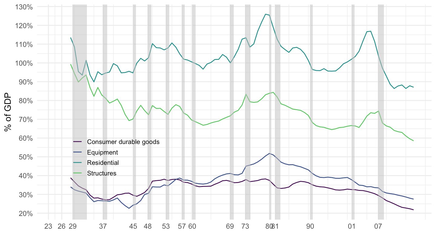
Figure B.4: U.S. Main Fixed Asset Components (1929-2017). Source: Fixed Asset Table 1.1 (BEA)

Figure B.5: Decomposition of Equipment (% of GDP). Source: Fixed Asset Table 2.1 (BEA)
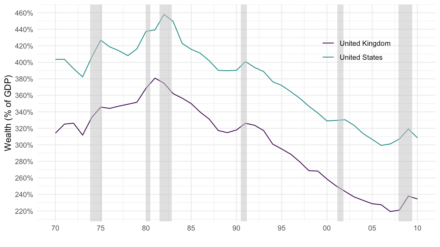
Figure B.6: Simulated 1970-2010 national wealth (% of national income) - savings flows
B.3 Investment
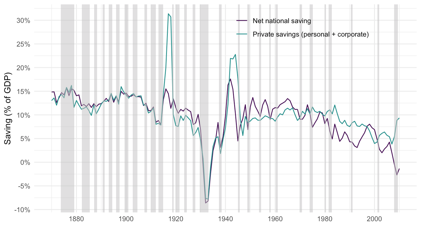
Figure B.7: U.S. Saving
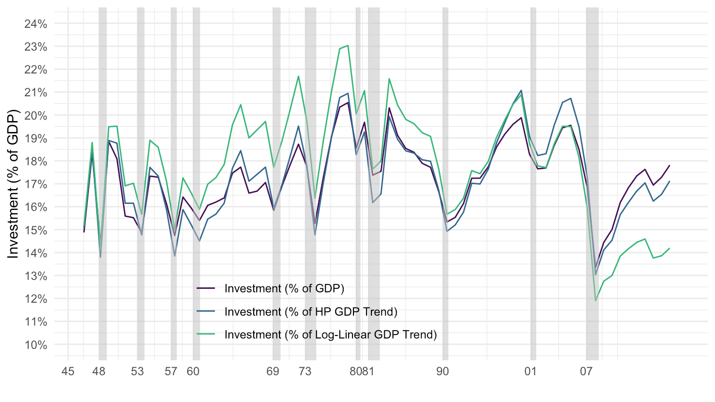
Figure B.8: U.S. Investment (% of GDP).

Figure B.9: Main Components of Investment (% of GDP) Source: Fixed Asset Table 1.5 (BEA)

Figure B.10: Decomposition of Equipment Investment (% of GDP). Source: Fixed Asset Table 2.7 (BEA)

Figure B.11: Decomposition of Structures Investment (% of GDP). Source: Fixed Asset Table 2.7 (BEA)
B.4 U.S. Budget Surpluses / Deficits
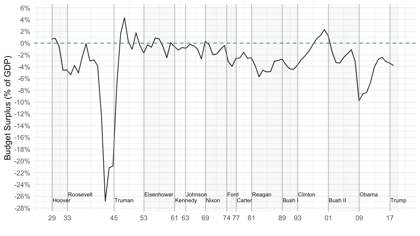
Figure B.12: Budget Surplus, 1929-2019 (% of GDP).
B.5 Net Exports
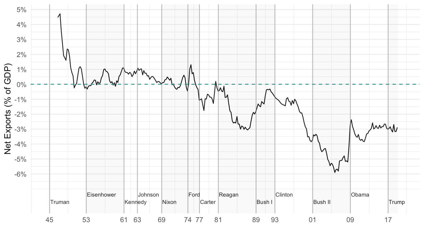
Figure B.13: Net Exports (% of GDP).
B.6 Effects of Rise in Public Saving (Romer and Romer (2010))
Figure B.14: GDP (Real) after a 1% of GDP increase in taxes (Romer and Romer (2010))
Figure B.15: Consumption (Real) after a 1% of GDP increase in taxes (Romer and Romer (2010))
Figure B.16: Investment (Real) after a 1% of GDP increase in taxes (Romer and Romer (2010))
Figure B.17: Unemployment after a 1% of GDP increase in taxes (Romer and Romer (2010))
Figure B.18: Residential Investment (Real)
Figure B.19: Real Imports
B.7 Real Effects of Monetary Policy Shocks (Romer and Romer (2004))
Figure B.20: GDP (Real) after a 1% increase in the Fed Funds Rate (Romer and Romer (2004))
Figure B.21: Unemployment
Figure B.22: Employment
Figure B.23: Real Consumption
Figure B.24: Real Imports
Figure B.25: Investment
Figure B.26: Production of Total Construction
Figure B.27: House Prices
B.8 Germany - Gerhard Schröder’s restrictive policies (1998-2003)
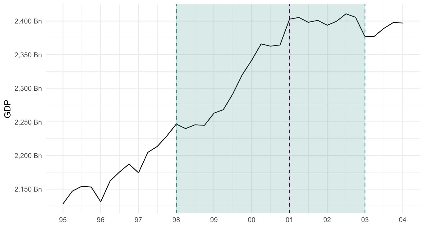
Figure B.28: GDP in Germany (1995-2004)
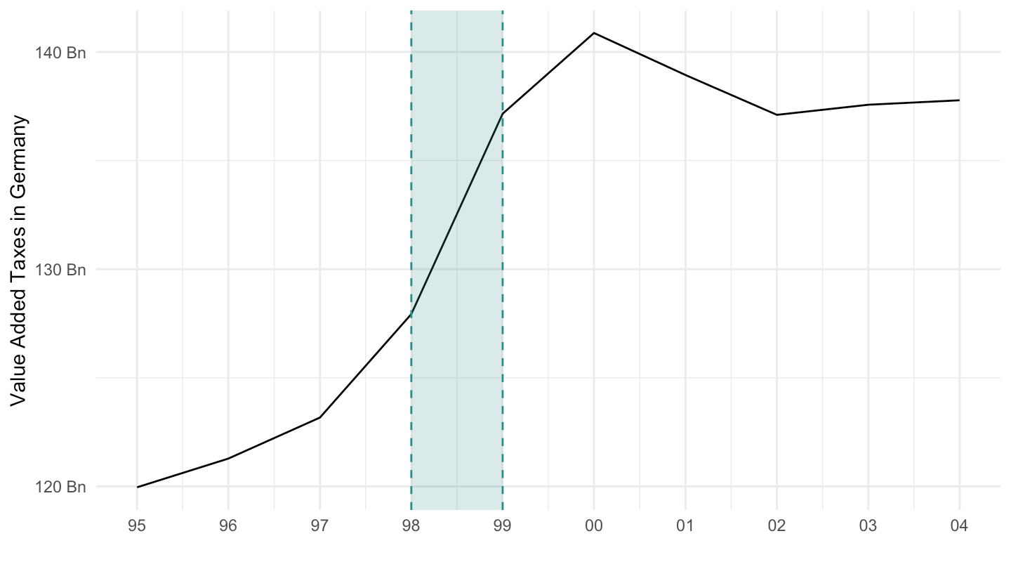
Figure B.29: Value Added Taxes in Germany (1995-2004)

Figure B.30: Fuel Taxes in Germany (1995-2004)
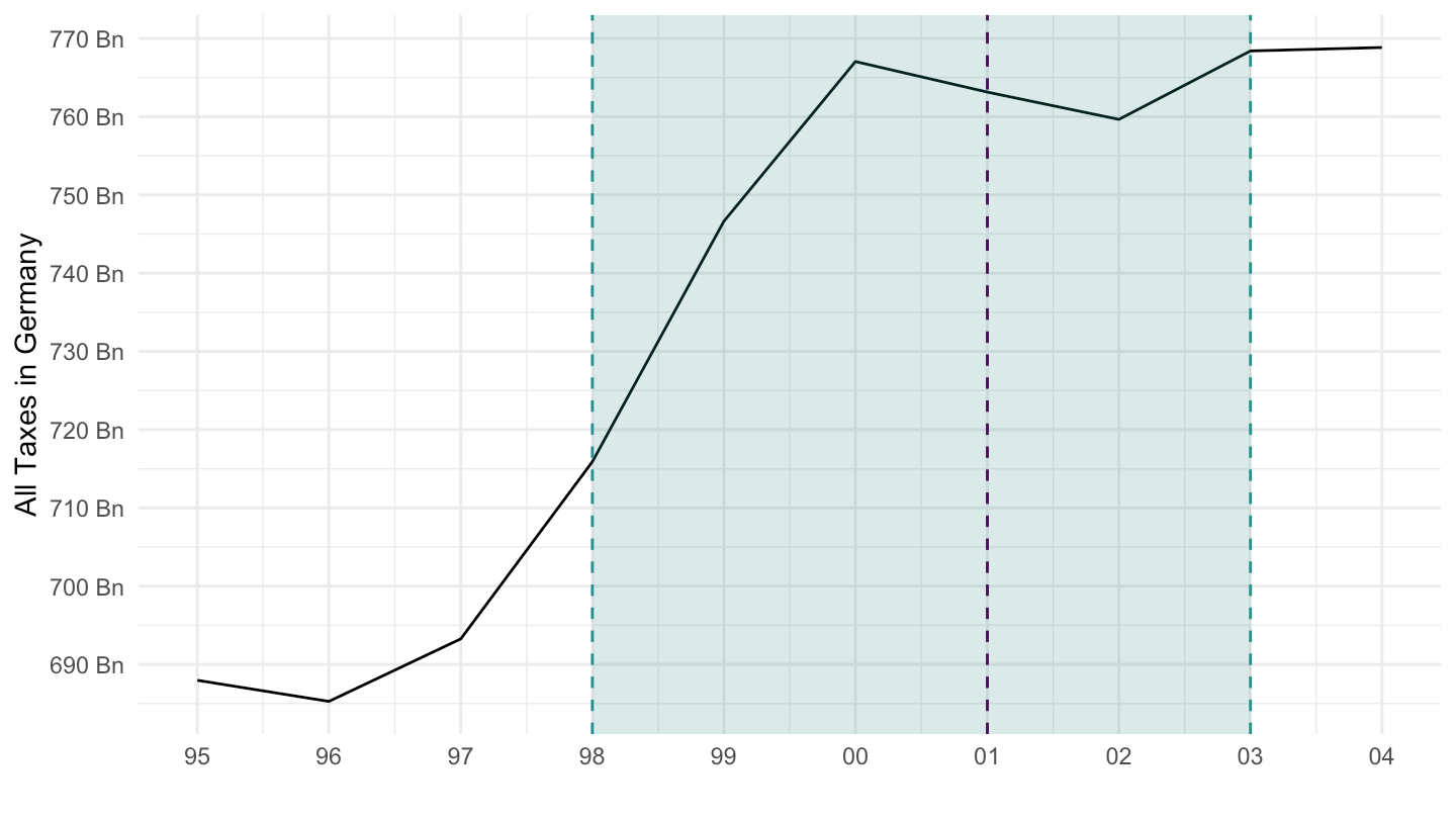
Figure B.31: Total Taxes in Germany (1995-2004)

Figure B.32: Consumption in Germany (1995-2004)
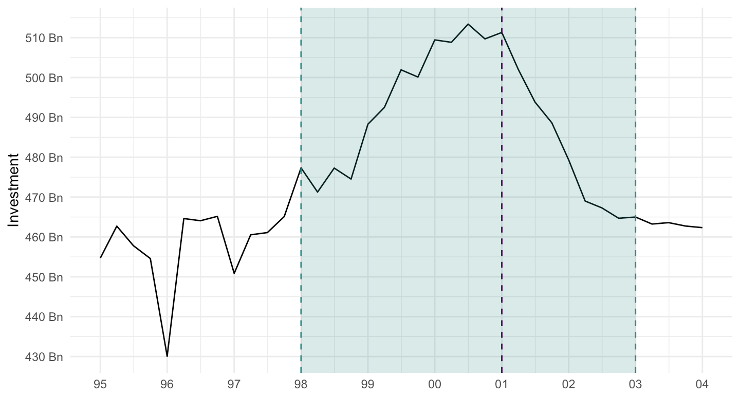
Figure B.33: Investment in Germany (1995-2004)
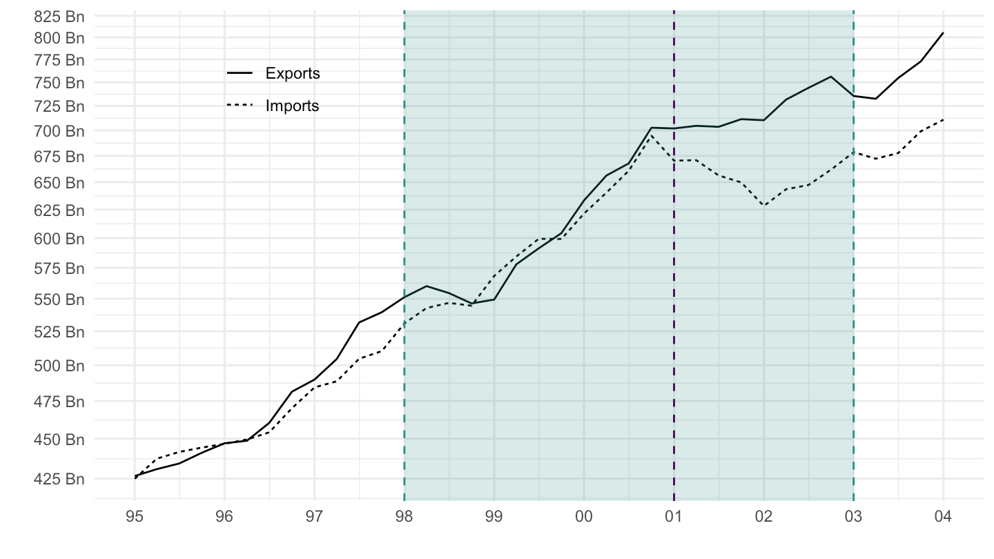
Figure B.34: Exports and Imports in Germany (1995-2004)
B.9 Japan’s boom-bust

Figure B.35: Real GDP
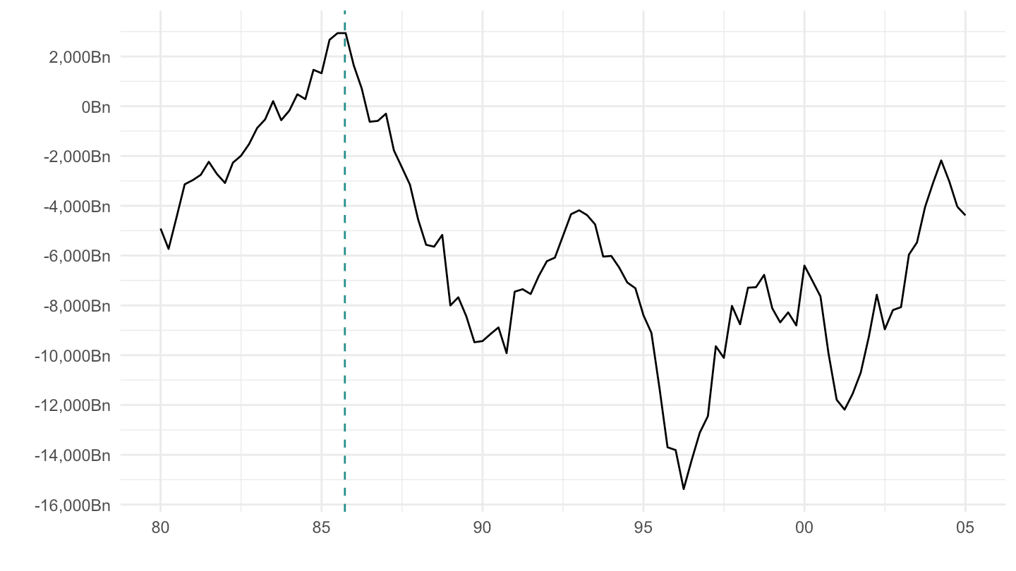
Figure B.36: Net Exports (1980-2005); September 22, 1985: Plaza Accords
C Tables
C.1 Capital
Table C.1 shows that the book value of capital is mostly composed of structures, and residential structures. This is important for thinking of capital / labor substitution, which is more intuitive for equipment.
| Description | 2017 |
|---|---|
| Fixed assets and consumer durable goods | 267% |
| Fixed assets | 245.2% |
| Private | 186.3% |
| Nonresidential | 99.3% |
| Equipment | 27.5% |
| Structures | 58.5% |
| IPP | 13.2% |
| Residential | 87.1% |
| Government | 58.9% |
| Nonresidential | 57.1% |
| Equipment | 4.2% |
| Structures | 48.1% |
| IPP | 4.8% |
| Residential | 1.8% |
| Consumer durable goods | 21.8% |
Even among equipment capital, many items do not in fact correspond to capital which can be thought of as being use in replacement for labor, as Table C.2 shows.
| Description | 2017 |
|---|---|
| Private fixed assets | 186.3% |
| Equipment | 27.7% |
| Nonresidential equipment | 27.5% |
| Information processing equipment | 6.3% |
| Computers and peripheral equipment | 1% |
| Communication equipment | 2.3% |
| Medical equipment and instruments | 1.8% |
| Nonmedical instruments | 0.9% |
| Photocopy and related equipment | 0.2% |
| Office and accounting equipment | 0% |
| Industrial equipment | 8.6% |
| Fabricated metal products | 0.7% |
| Engines and turbines | 0.6% |
| Metalworking machinery | 1.2% |
| Special industry machinery, n.e.c. | 1.4% |
| General industrial, including materials handling, equipment | 2.7% |
| Electrical transmission, distribution, and industrial apparatus | 2.1% |
| Transportation equipment | 6.3% |
| Trucks, buses, and truck trailers | 2.6% |
| Light trucks (including utility vehicles) | 1.7% |
| Other trucks, buses, and truck trailers | 0.9% |
| Autos | 0.8% |
| Aircraft | 1.8% |
| Ships and boats | 0.4% |
| Railroad equipment | 0.7% |
| Other equipment | 6.3% |
| Furniture and fixtures | 1.4% |
| Agricultural machinery | 0.9% |
| Construction machinery | 1% |
| Mining and oilfield machinery | 0.6% |
| Service industry machinery | 0.8% |
| Electrical equipment, n.e.c. | 0.1% |
| Other nonresidential equipment | 1.5% |
| Residential equipment | 0.2% |
Email: fgeerolf@econ.ucla.edu↩
First version: May 2012. This is a much revised version from Chapter 1 of my 2013 Ph.D. dissertation at Sciences Po Paris. I thank Emmanuel Farhi, Christian Gollier, Pierre-Olivier Gourinchas, Christian Hellwig, Greg Mankiw, Philippe Martin, Thomas Piketty, Ken Rogoff, Larry Summers, Andrei Shleifer, Jean Tirole, Jaume Ventura, Philippe Weil, Richard Zeckhauser, Gabriel Zucman and seminar participants at Collège de France, Harvard University, INSEE-CREST, MIT and at the Sveriges Riksbank Conference on Bubbles for comments and suggestions. I am grateful to Harvard University and the Massachusetts Institute of Technology, where part of this research was carried out, for their hospitality.↩