
Last observation: 2020 (N = 40876)
First observation: 1970 (N = 8658)
Last data update: 02 août 2026, 09:08
Last compile: 09 oct. 2026, 23:46
SHA |>
  group_by(obsTime) |>
  summarise(Nobs = n()) |>
  arrange(desc(obsTime)) |>
print_table_conditional()SHA |>
filter(MEASURE == "PARPIB",
HP == "HPTOT",
HF == "HFTOT",
LOCATION %in% c("FRA", "DEU", "KOR", "USA")) |>
left_join(SHA_var$HC, by = "HC") |>
group_by(LOCATION, HC, Hc) |>
summarise(value = last(obsValue)) |>
spread(LOCATION, value) |>
print_table_conditional()SHA |>
filter(MEASURE == "PARPIB",
HP == "HPTOT",
HC == "HCTOT",
LOCATION %in% c("FRA", "DEU", "ITA")) |>
left_join(SHA_var$HF, by = "HF") |>
group_by(LOCATION, HF, Hf) |>
summarise(value = last(obsValue)) |>
spread(LOCATION, value) |>
print_table_conditional()| HF | Hf | DEU | FRA | ITA |
|---|---|---|---|---|
| HF1 | Government/compulsory schemes | 10.665 | 9.302 | 7.412 |
| HF11 | Government schemes | 0.764 | 0.612 | 7.395 |
| HF121 | Social health insurance schemes | 8.292 | 7.938 | 0.016 |
| HF122 | Compulsory private insurance schemes | 0.841 | 0.751 | NA |
| HF12HF13 | Compulsory contributory health insurance schemes | 9.132 | 8.689 | 0.016 |
| HF2 | Voluntary health care payment schemes | 0.323 | 0.781 | 0.252 |
| HF21 | Voluntary health insurance schemes | 0.163 | 0.712 | 0.191 |
| HF22 | NPISH financing schemes | 0.105 | 0.001 | 0.020 |
| HF23 | Enterprise financing schemes | 0.048 | 0.069 | 0.040 |
| HF2HF3 | Voluntary schemes/household out-of-pocket payments | 1.865 | 1.810 | 2.304 |
| HF3 | Household out-of-pocket payments | 1.542 | 1.029 | 2.053 |
| HF31 | Out-of-pocket excluding cost-sharing | NA | 0.530 | NA |
| HF32 | Cost-sharing with third-party payers | NA | 0.499 | NA |
| HFTOT | All financing schemes | 12.530 | 12.377 | 9.716 |
SHA |>
  filter(HC == "HCTOT",
         MEASURE == "PARPIB",
         HP == "HPTOT",
         HF == "HFTOT",
         LOCATION %in% c("FRA", "DEU", "ITA")) |>
  left_join(SHA_var$LOCATION, by = "LOCATION") |>
  year_to_date() |>
  add_flag_color("Location") |>
  mutate(obsValue = obsValue/100) |>
  ggplot() + geom_line(aes(x = date, y = obsValue, color = color)) +
  scale_color_identity() + theme_minimal() + add_3flags +
  scale_x_date(breaks = seq(1920, 2100, 5) |> paste0("-01-01") |> as.Date(),
               labels = date_format("%Y")) +
  scale_y_continuous(breaks = 0.01*seq(-7, 60, 1),
                     labels = scales::percent_format(accuracy = 1)) +
  ylab("% of GDP") + xlab("")
SHA |>
  filter(HC == "HCTOT",
         MEASURE == "PARPIB",
         HP == "HPTOT",
         HF == "HF1",
         LOCATION %in% c("FRA", "DEU", "ITA")) |>
  left_join(SHA_var$LOCATION, by = "LOCATION") |>
  year_to_date() |>
  add_flag_color("Location") |>
  mutate(obsValue = obsValue/100) |>
  ggplot() + geom_line(aes(x = date, y = obsValue, color = color)) +
  scale_color_identity() + theme_minimal() + add_3flags +
  scale_x_date(breaks = seq(1920, 2100, 5) |> paste0("-01-01") |> as.Date(),
               labels = date_format("%Y")) +
  scale_y_continuous(breaks = 0.01*seq(-7, 60, 1),
                     labels = scales::percent_format(accuracy = 1)) +
  ylab("% of GDP") + xlab("")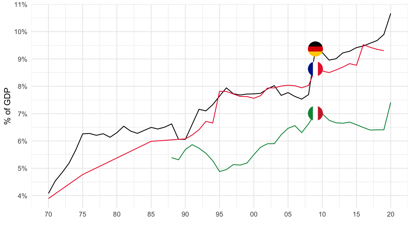
SHA |>
  filter(HC == "HCTOT",
         MEASURE == "PARPIB",
         HP == "HPTOT",
         HF == "HF11",
         LOCATION %in% c("FRA", "DEU", "ITA")) |>
  left_join(SHA_var$LOCATION, by = "LOCATION") |>
  year_to_date() |>
  add_flag_color("Location") |>
  mutate(obsValue = obsValue/100) |>
  ggplot() + geom_line(aes(x = date, y = obsValue, color = color)) +
  scale_color_identity() + theme_minimal() + add_3flags +
  scale_x_date(breaks = seq(1920, 2100, 5) |> paste0("-01-01") |> as.Date(),
               labels = date_format("%Y")) +
  scale_y_continuous(breaks = 0.01*seq(-7, 60, 1),
                     labels = scales::percent_format(accuracy = 1)) +
  ylab("% of GDP") + xlab("")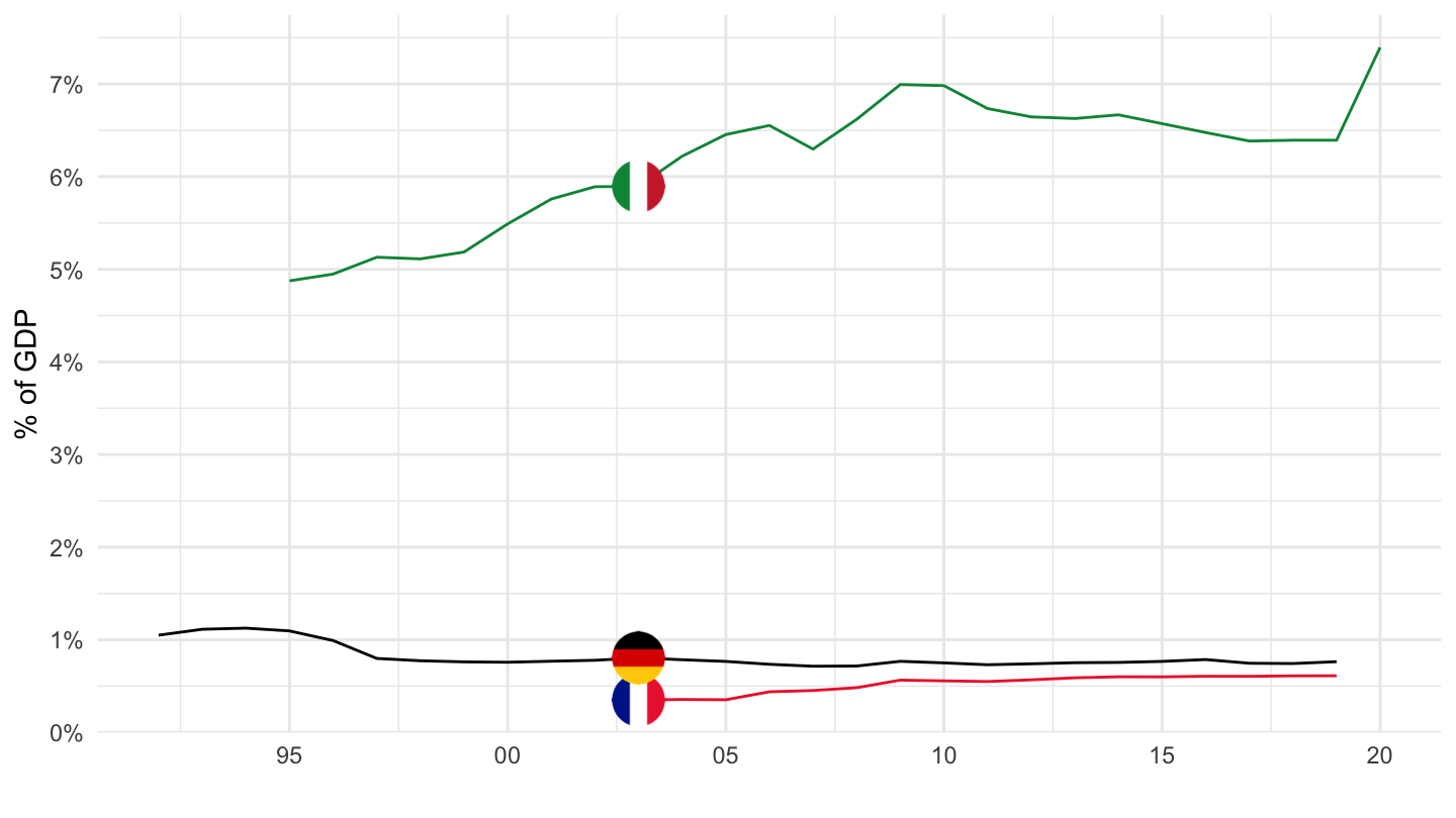
SHA |>
  filter(HC == "HCTOT",
         MEASURE == "PARPIB",
         HP == "HPTOT",
         HF == "HF121",
         LOCATION %in% c("FRA", "DEU", "ITA")) |>
  left_join(SHA_var$LOCATION, by = "LOCATION") |>
  year_to_date() |>
  add_flag_color("Location") |>
  mutate(obsValue = obsValue/100) |>
  ggplot() + geom_line(aes(x = date, y = obsValue, color = color)) +
  scale_color_identity() + theme_minimal() + add_3flags +
  scale_x_date(breaks = seq(1920, 2100, 5) |> paste0("-01-01") |> as.Date(),
               labels = date_format("%Y")) +
  scale_y_continuous(breaks = 0.01*seq(-7, 60, 1),
                     labels = scales::percent_format(accuracy = 1)) +
  ylab("% of GDP") + xlab("")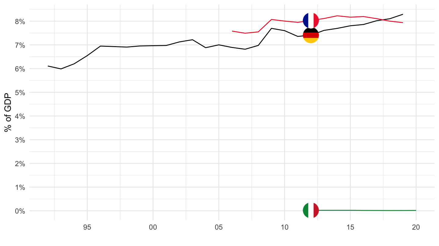
SHA |>
  filter(HC == "HCTOT",
         MEASURE == "PARPIB",
         HP == "HPTOT",
         HF == "HF122",
         LOCATION %in% c("FRA", "DEU", "ITA")) |>
  left_join(SHA_var$LOCATION, by = "LOCATION") |>
  year_to_date() |>
  add_flag_color("Location") |>
  mutate(obsValue = obsValue/100) |>
  ggplot() + geom_line(aes(x = date, y = obsValue, color = color)) +
  scale_color_identity() + theme_minimal() + add_3flags +
  scale_x_date(breaks = seq(1920, 2100, 5) |> paste0("-01-01") |> as.Date(),
               labels = date_format("%Y")) +
  scale_y_continuous(breaks = 0.01*seq(-7, 60, .1),
                     labels = scales::percent_format(accuracy = .1)) +
  ylab("% of GDP") + xlab("")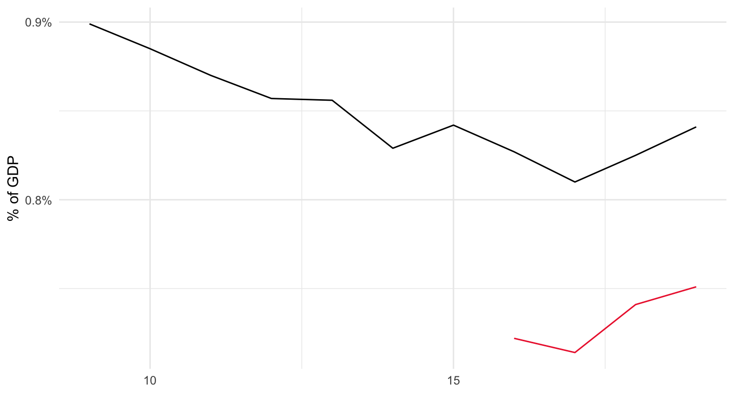
SHA |>
  filter(HC == "HCTOT",
         MEASURE == "PARPIB",
         HP == "HPTOT",
         HF == "HF2HF3",
         LOCATION %in% c("FRA", "DEU", "ITA")) |>
  left_join(SHA_var$LOCATION, by = "LOCATION") |>
  year_to_date() |>
  add_flag_color("Location") |>
  mutate(obsValue = obsValue/100) |>
  ggplot() + geom_line(aes(x = date, y = obsValue, color = color)) +
  scale_color_identity() + theme_minimal() + add_3flags +
  scale_x_date(breaks = seq(1920, 2100, 5) |> paste0("-01-01") |> as.Date(),
               labels = date_format("%Y")) +
  scale_y_continuous(breaks = 0.01*seq(-7, 60, 0.2),
                     labels = scales::percent_format(accuracy = .1)) +
  ylab("% of GDP") + xlab("")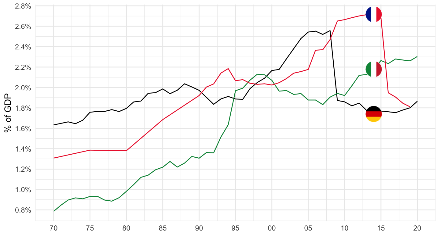
SHA |>
  filter(HC == "HCTOT",
         MEASURE == "PARPIB",
         HP == "HPTOT",
         HF == "HF2",
         LOCATION %in% c("FRA", "DEU", "ITA")) |>
  left_join(SHA_var$LOCATION, by = "LOCATION") |>
  year_to_date() |>
  add_flag_color("Location") |>
  mutate(obsValue = obsValue/100) |>
  ggplot() + geom_line(aes(x = date, y = obsValue, color = color)) +
  scale_color_identity() + theme_minimal() + add_3flags +
  scale_x_date(breaks = seq(1920, 2100, 5) |> paste0("-01-01") |> as.Date(),
               labels = date_format("%Y")) +
  scale_y_continuous(breaks = 0.01*seq(-7, 60, 0.2),
                     labels = scales::percent_format(accuracy = .1)) +
  ylab("% of GDP") + xlab("")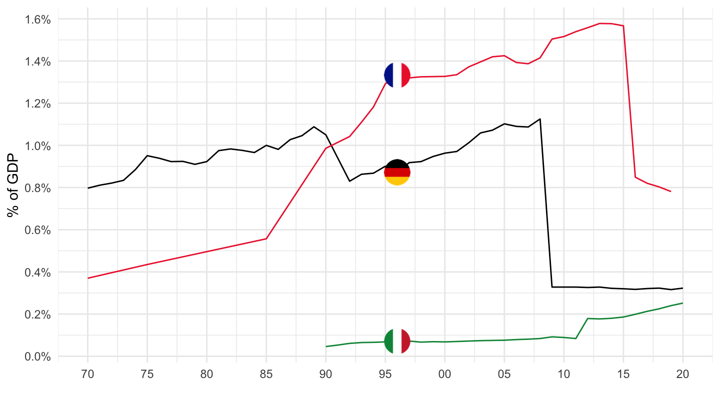
SHA |>
  filter(HC == "HCTOT",
         MEASURE == "PARPIB",
         HP == "HPTOT",
         HF == "HF21",
         LOCATION %in% c("FRA", "DEU", "ITA")) |>
  left_join(SHA_var$LOCATION, by = "LOCATION") |>
  year_to_date() |>
  add_flag_color("Location") |>
  mutate(obsValue = obsValue/100) |>
  ggplot() + geom_line(aes(x = date, y = obsValue, color = color)) +
  scale_color_identity() + theme_minimal() + add_3flags +
  scale_x_date(breaks = seq(1920, 2100, 5) |> paste0("-01-01") |> as.Date(),
               labels = date_format("%Y")) +
  scale_y_continuous(breaks = 0.01*seq(-7, 60, 0.2),
                     labels = scales::percent_format(accuracy = .1)) +
  ylab("% of GDP") + xlab("")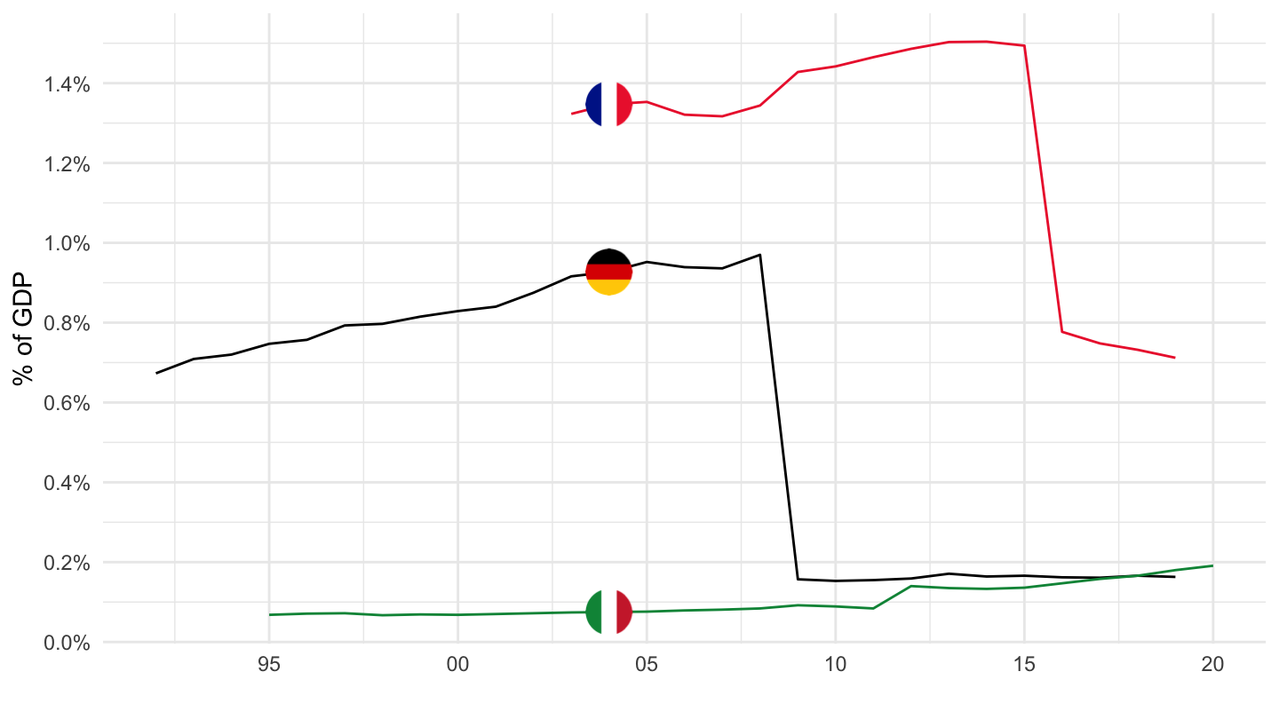
SHA |>
  filter(HC == "HCTOT",
         MEASURE == "PARPIB",
         HP == "HPTOT",
         HF == "HF22",
         LOCATION %in% c("FRA", "DEU", "ITA")) |>
  left_join(SHA_var$LOCATION, by = "LOCATION") |>
  year_to_date() |>
  add_flag_color("Location") |>
  mutate(obsValue = obsValue/100) |>
  ggplot() + geom_line(aes(x = date, y = obsValue, color = color)) +
  scale_color_identity() + theme_minimal() + add_3flags +
  scale_x_date(breaks = seq(1920, 2100, 5) |> paste0("-01-01") |> as.Date(),
               labels = date_format("%Y")) +
  scale_y_continuous(breaks = 0.01*seq(-7, 60, 0.01),
                     labels = scales::percent_format(accuracy = .01)) +
  ylab("% of GDP") + xlab("")
SHA |>
  filter(HC == "HCTOT",
         MEASURE == "PARPIB",
         HP == "HPTOT",
         HF == "HF23",
         LOCATION %in% c("FRA", "DEU", "ITA")) |>
  left_join(SHA_var$LOCATION, by = "LOCATION") |>
  year_to_date() |>
  add_flag_color("Location") |>
  mutate(obsValue = obsValue/100) |>
  ggplot() + geom_line(aes(x = date, y = obsValue, color = color)) +
  scale_color_identity() + theme_minimal() + add_3flags +
  scale_x_date(breaks = seq(1920, 2100, 5) |> paste0("-01-01") |> as.Date(),
               labels = date_format("%Y")) +
  scale_y_continuous(breaks = 0.01*seq(-7, 60, 0.01),
                     labels = scales::percent_format(accuracy = .01)) +
  ylab("% of GDP") + xlab("")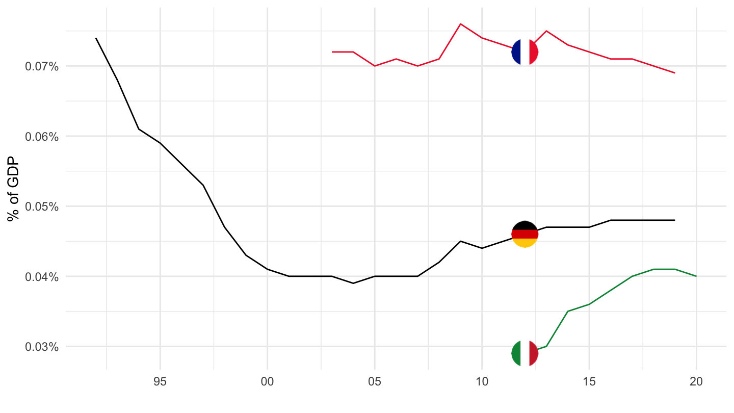
SHA |>
  filter(HC == "HCTOT",
         MEASURE == "PARPIB",
         HP == "HPTOT",
         HF == "HF3",
         LOCATION %in% c("FRA", "DEU", "ITA")) |>
  left_join(SHA_var$LOCATION, by = "LOCATION") |>
  year_to_date() |>
  add_flag_color("Location") |>
  mutate(obsValue = obsValue/100) |>
  ggplot() + geom_line(aes(x = date, y = obsValue, color = color)) +
  scale_color_identity() + theme_minimal() + add_3flags +
  scale_x_date(breaks = seq(1920, 2100, 5) |> paste0("-01-01") |> as.Date(),
               labels = date_format("%Y")) +
  scale_y_continuous(breaks = 0.01*seq(-7, 60, 0.2),
                     labels = scales::percent_format(accuracy = .1)) +
  ylab("% of GDP") + xlab("")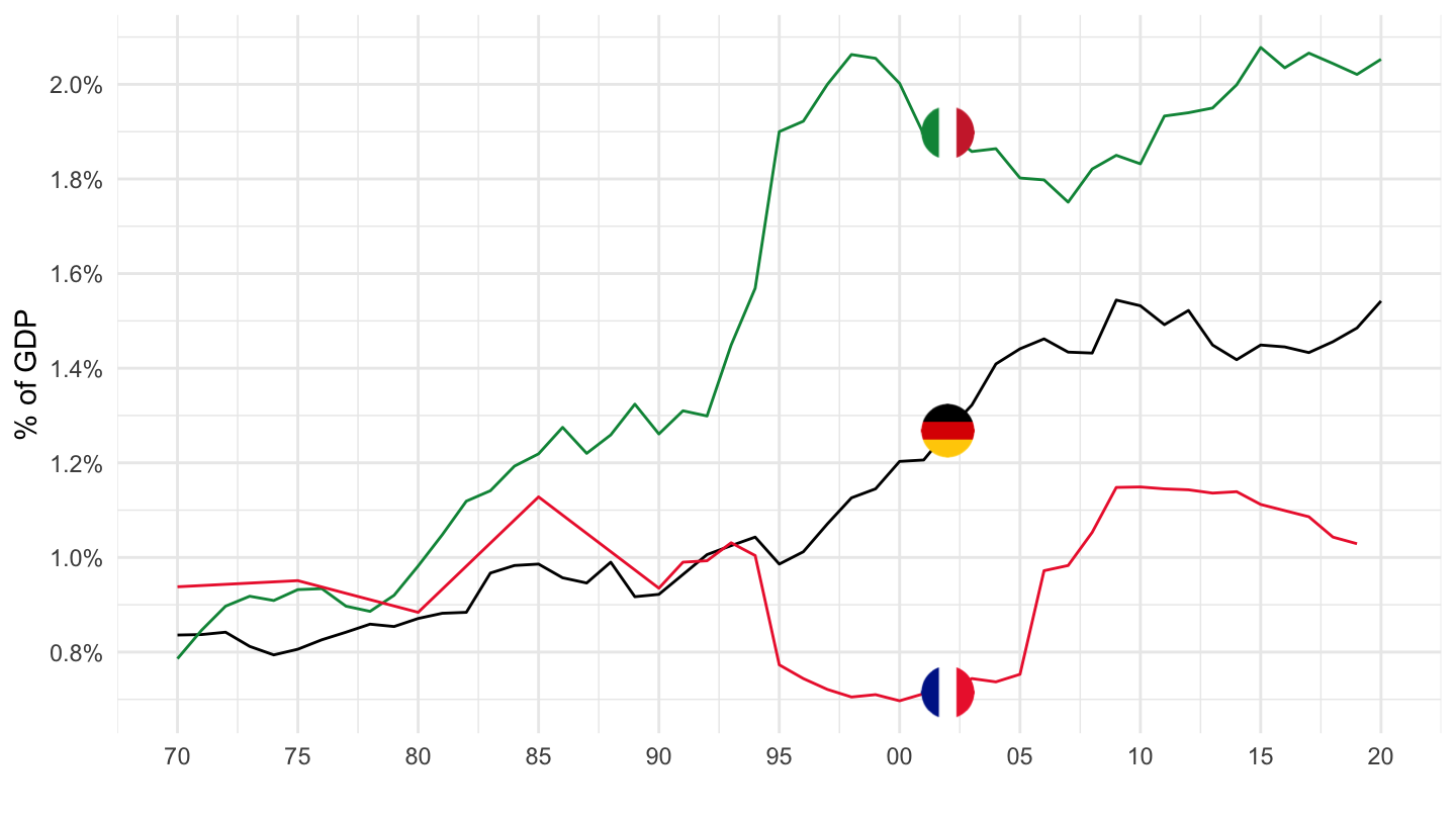
SHA |>
  filter(HC == "HCTOT",
         MEASURE == "PARPIB",
         HP == "HPTOT",
         HF == "HF31",
         LOCATION %in% c("FRA", "DEU", "ITA")) |>
  left_join(SHA_var$LOCATION, by = "LOCATION") |>
  year_to_date() |>
  add_flag_color("Location") |>
  mutate(obsValue = obsValue/100) |>
  ggplot() + geom_line(aes(x = date, y = obsValue, color = color)) +
  scale_color_identity() + theme_minimal() + add_3flags +
  scale_x_date(breaks = seq(1920, 2100, 1) |> paste0("-01-01") |> as.Date(),
               labels = date_format("%Y")) +
  scale_y_continuous(breaks = 0.01*seq(-7, 60, 0.01),
                     labels = scales::percent_format(accuracy = .01)) +
  ylab("% of GDP") + xlab("")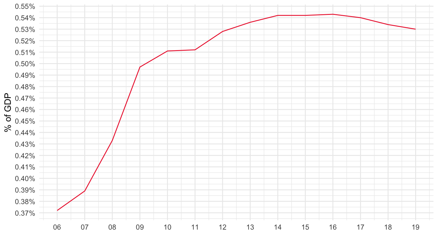
SHA |>
  filter(HC == "HCTOT",
         MEASURE == "PARPIB",
         HP == "HPTOT",
         HF == "HF32",
         LOCATION %in% c("FRA", "DEU", "ITA")) |>
  left_join(SHA_var$LOCATION, by = "LOCATION") |>
  year_to_date() |>
  add_flag_color("Location") |>
  mutate(obsValue = obsValue/100) |>
  ggplot() + geom_line(aes(x = date, y = obsValue, color = color)) +
  scale_color_identity() + theme_minimal() + add_3flags +
  scale_x_date(breaks = seq(1920, 2100, 1) |> paste0("-01-01") |> as.Date(),
               labels = date_format("%Y")) +
  scale_y_continuous(breaks = 0.01*seq(-7, 60, 0.01),
                     labels = scales::percent_format(accuracy = .01)) +
  ylab("% of GDP") + xlab("")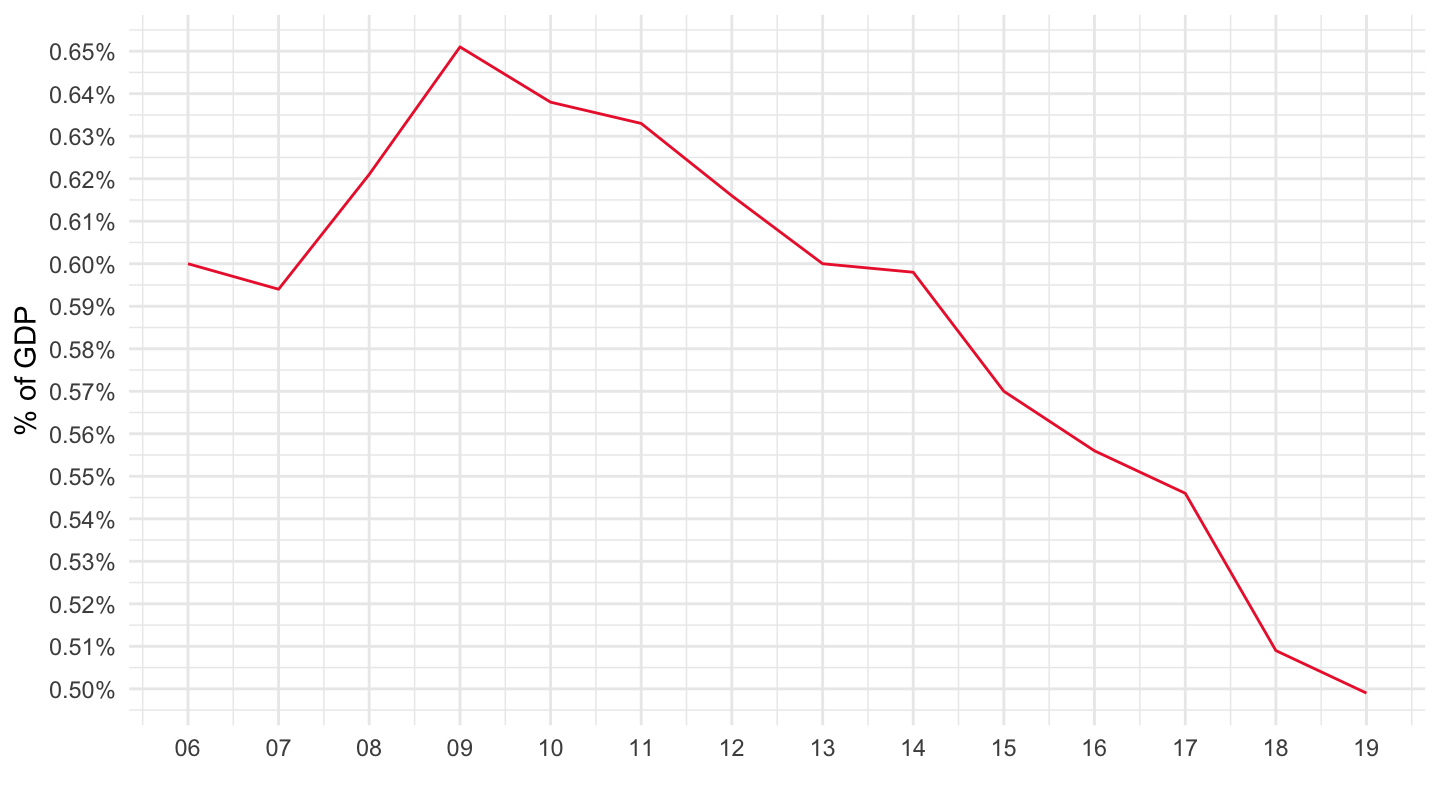
SHA |>
  filter(HC == "HC6",
         MEASURE == "PARPIB",
         HP == "HPTOT",
         HF == "HFTOT") |>
  left_join(SHA_var$LOCATION, by = "LOCATION") |>
  group_by(LOCATION, Location) |>
  summarise(Nobs = n(),
            `Year 1` = first(obsTime),
            `Preventive Care 1` = first(obsValue),
            `Year 2` = last(obsTime),
            `Preventive Care 2` = last(obsValue)) |>
  arrange(-`Preventive Care 2`) |>
print_table_conditional()SHA |>
filter(HC == "HC6",
MEASURE == "PARPIB",
HP == "HPTOT",
HF == "HFTOT",
LOCATION %in% c("FRA", "DEU", "KOR")) |>
left_join(SHA_var$LOCATION, by = "LOCATION") |>
year_to_date() |>
add_flag_color("Location") |>
mutate(obsValue = obsValue/100) |>
ggplot() + geom_line(aes(x = date, y = obsValue, color = color)) +
scale_color_identity() + theme_minimal() + add_3flags +
scale_x_date(breaks = seq(1920, 2100, 5) |> paste0("-01-01") |> as.Date(),
labels = date_format("%Y")) +
scale_y_continuous(breaks = 0.01*seq(-7, 60, 0.05),
labels = scales::percent_format(accuracy = 0.01)) +
ylab("Preventive Care (% of GDP)") + xlab("")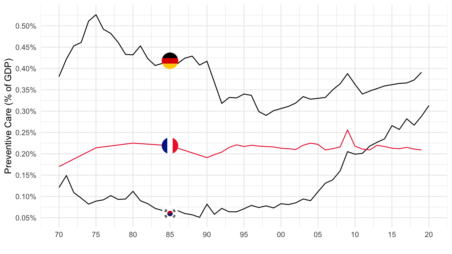
SHA |>
  filter(HC == "HC62",
         MEASURE == "PARPIB",
         HP == "HPTOT",
         HF == "HFTOT") |>
  left_join(SHA_var$LOCATION, by = "LOCATION") |>
  group_by(LOCATION, Location) |>
  summarise(Nobs = n(),
            `Year 1` = first(obsTime),
            `Immunisation 1 (% of GDP)` = first(obsValue),
            `Year 2` = last(obsTime),
            `Immunisation 2 (% of GDP)` = last(obsValue)) |>
  arrange(-`Immunisation 2 (% of GDP)`) |>
print_table_conditional()| LOCATION | Location | Nobs | Year 1 | Immunisation 1 (% of GDP) | Year 2 | Immunisation 2 (% of GDP) |
|---|---|---|---|---|---|---|
| COL | Colombia | 5 | 2013 | 0.125 | 2017 | 0.133 |
| BRA | Brazil | 5 | 2015 | 0.076 | 2019 | 0.108 |
| DEU | Germany | 28 | 1992 | 0.025 | 2019 | 0.064 |
| ISL | Iceland | 18 | 2003 | 0.070 | 2020 | 0.053 |
| SWE | Sweden | 19 | 2001 | 0.035 | 2019 | 0.049 |
| SVN | Slovenia | 7 | 2012 | 0.035 | 2019 | 0.047 |
| GBR | United Kingdom | 7 | 2013 | 0.039 | 2019 | 0.041 |
| KOR | Korea | 37 | 1970 | 0.001 | 2020 | 0.040 |
| LVA | Latvia | 7 | 2013 | 0.031 | 2019 | 0.034 |
| LTU | Lithuania | 14 | 2006 | 0.006 | 2019 | 0.031 |
| CZE | Czech Republic | 7 | 2013 | 0.081 | 2019 | 0.029 |
| RUS | Russia | 5 | 2015 | 0.013 | 2019 | 0.021 |
| MEX | Mexico | 17 | 2003 | 0.016 | 2019 | 0.020 |
| DNK | Denmark | 10 | 2010 | 0.006 | 2019 | 0.018 |
| EST | Estonia | 8 | 2012 | 0.028 | 2019 | 0.014 |
| FIN | Finland | 21 | 2000 | 0.004 | 2020 | 0.013 |
| LUX | Luxembourg | 9 | 2011 | 0.018 | 2019 | 0.013 |
| GRC | Greece | 17 | 2003 | 0.005 | 2019 | 0.007 |
| POL | Poland | 7 | 2013 | 0.007 | 2019 | 0.007 |
| CRI | Costa Rica | 9 | 2011 | 0.005 | 2019 | 0.006 |
| FRA | France | 14 | 2006 | 0.004 | 2019 | 0.006 |
| BEL | Belgium | 17 | 2003 | 0.003 | 2019 | 0.002 |
SHA |>
  filter(HC == "HC62",
         MEASURE == "PARPIB",
         HP == "HPTOT",
         HF == "HFTOT",
         LOCATION %in% c("FRA", "DEU", "KOR")) |>
  left_join(SHA_var$LOCATION, by = "LOCATION") |>
  year_to_date() |>
  add_flag_color("Location") |>
  mutate(obsValue = obsValue/100) |>
  ggplot() + geom_line(aes(x = date, y = obsValue, color = color)) +
  scale_color_identity() + theme_minimal() + add_3flags +
  scale_x_date(breaks = seq(1920, 2100, 5) |> paste0("-01-01") |> as.Date(),
               labels = date_format("%Y")) +
  scale_y_continuous(breaks = 0.01*seq(-7, 60, 0.01),
                     labels = scales::percent_format(accuracy = 0.01)) +
  ylab("Immunisation (% of GDP)") + xlab("")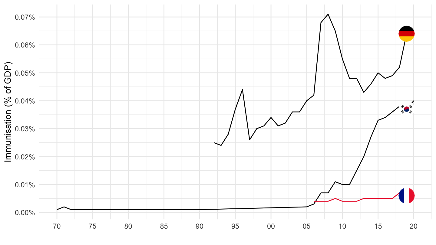
SHA |>
  filter(HC == "HC62",
         MEASURE == "PARPIB",
         HP == "HPTOT",
         HF == "HFTOT") |>
  left_join(SHA_var$LOCATION, by = "LOCATION") |>
  group_by(LOCATION, Location) |>
  summarise(Nobs = n(),
            `Year 1` = first(obsTime),
            `Early Detection 1 (% of GDP)` = first(obsValue),
            `Year 2` = last(obsTime),
            `Early Detection 2 (% of GDP)` = last(obsValue)) |>
  arrange(-`Early Detection 2 (% of GDP)`) |>
print_table_conditional()| LOCATION | Location | Nobs | Year 1 | Early Detection 1 (% of GDP) | Year 2 | Early Detection 2 (% of GDP) |
|---|---|---|---|---|---|---|
| COL | Colombia | 5 | 2013 | 0.125 | 2017 | 0.133 |
| BRA | Brazil | 5 | 2015 | 0.076 | 2019 | 0.108 |
| DEU | Germany | 28 | 1992 | 0.025 | 2019 | 0.064 |
| ISL | Iceland | 18 | 2003 | 0.070 | 2020 | 0.053 |
| SWE | Sweden | 19 | 2001 | 0.035 | 2019 | 0.049 |
| SVN | Slovenia | 7 | 2012 | 0.035 | 2019 | 0.047 |
| GBR | United Kingdom | 7 | 2013 | 0.039 | 2019 | 0.041 |
| KOR | Korea | 37 | 1970 | 0.001 | 2020 | 0.040 |
| LVA | Latvia | 7 | 2013 | 0.031 | 2019 | 0.034 |
| LTU | Lithuania | 14 | 2006 | 0.006 | 2019 | 0.031 |
| CZE | Czech Republic | 7 | 2013 | 0.081 | 2019 | 0.029 |
| RUS | Russia | 5 | 2015 | 0.013 | 2019 | 0.021 |
| MEX | Mexico | 17 | 2003 | 0.016 | 2019 | 0.020 |
| DNK | Denmark | 10 | 2010 | 0.006 | 2019 | 0.018 |
| EST | Estonia | 8 | 2012 | 0.028 | 2019 | 0.014 |
| FIN | Finland | 21 | 2000 | 0.004 | 2020 | 0.013 |
| LUX | Luxembourg | 9 | 2011 | 0.018 | 2019 | 0.013 |
| GRC | Greece | 17 | 2003 | 0.005 | 2019 | 0.007 |
| POL | Poland | 7 | 2013 | 0.007 | 2019 | 0.007 |
| CRI | Costa Rica | 9 | 2011 | 0.005 | 2019 | 0.006 |
| FRA | France | 14 | 2006 | 0.004 | 2019 | 0.006 |
| BEL | Belgium | 17 | 2003 | 0.003 | 2019 | 0.002 |
SHA |>
  filter(HC == "HC63",
         MEASURE == "PARPIB",
         HP == "HPTOT",
         HF == "HFTOT",
         LOCATION %in% c("FRA", "DEU", "KOR")) |>
  left_join(SHA_var$LOCATION, by = "LOCATION") |>
  year_to_date() |>
  add_flag_color("Location") |>
  mutate(obsValue = obsValue/100) |>
  ggplot() + geom_line(aes(x = date, y = obsValue, color = color)) +
  scale_color_identity() + theme_minimal() + add_3flags +
  scale_x_date(breaks = seq(1920, 2100, 5) |> paste0("-01-01") |> as.Date(),
               labels = date_format("%Y")) +
  scale_y_continuous(breaks = 0.01*seq(-7, 60, 0.01),
                     labels = scales::percent_format(accuracy = 0.01)) +
  ylab("Early disease detection programmes (% of GDP)") + xlab("")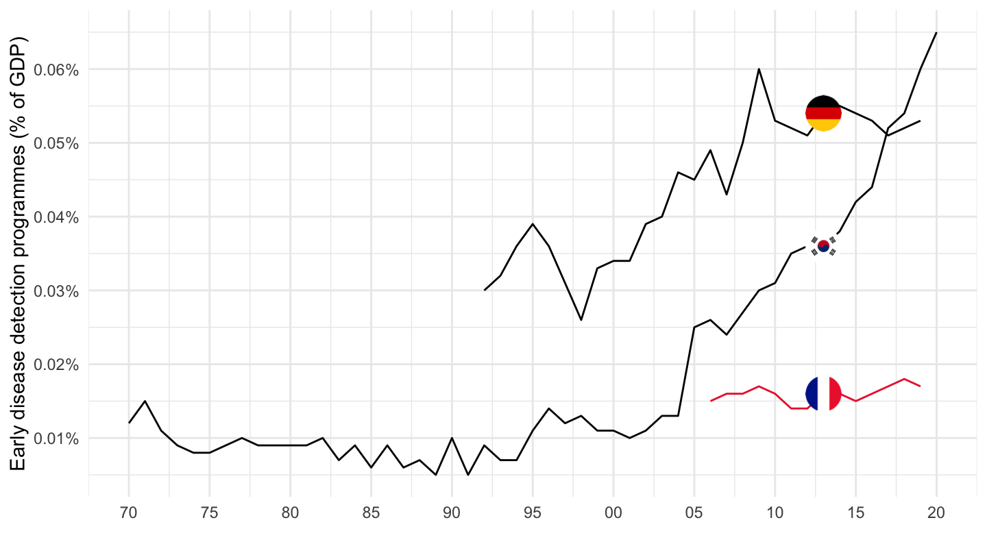
SHA |>
  filter(HC == "HC62",
         MEASURE == "PARPIB",
         HP == "HPTOT",
         HF == "HFTOT") |>
  left_join(SHA_var$LOCATION, by = "LOCATION") |>
  group_by(LOCATION, Location) |>
  summarise(Nobs = n(),
            `Year 1` = first(obsTime),
            `Surveillance 1 (% of GDP)` = first(obsValue),
            `Year 2` = last(obsTime),
            `Surveillance 2 (% of GDP)` = last(obsValue)) |>
  arrange(-`Surveillance 2 (% of GDP)`) |>
print_table_conditional()| LOCATION | Location | Nobs | Year 1 | Surveillance 1 (% of GDP) | Year 2 | Surveillance 2 (% of GDP) |
|---|---|---|---|---|---|---|
| COL | Colombia | 5 | 2013 | 0.125 | 2017 | 0.133 |
| BRA | Brazil | 5 | 2015 | 0.076 | 2019 | 0.108 |
| DEU | Germany | 28 | 1992 | 0.025 | 2019 | 0.064 |
| ISL | Iceland | 18 | 2003 | 0.070 | 2020 | 0.053 |
| SWE | Sweden | 19 | 2001 | 0.035 | 2019 | 0.049 |
| SVN | Slovenia | 7 | 2012 | 0.035 | 2019 | 0.047 |
| GBR | United Kingdom | 7 | 2013 | 0.039 | 2019 | 0.041 |
| KOR | Korea | 37 | 1970 | 0.001 | 2020 | 0.040 |
| LVA | Latvia | 7 | 2013 | 0.031 | 2019 | 0.034 |
| LTU | Lithuania | 14 | 2006 | 0.006 | 2019 | 0.031 |
| CZE | Czech Republic | 7 | 2013 | 0.081 | 2019 | 0.029 |
| RUS | Russia | 5 | 2015 | 0.013 | 2019 | 0.021 |
| MEX | Mexico | 17 | 2003 | 0.016 | 2019 | 0.020 |
| DNK | Denmark | 10 | 2010 | 0.006 | 2019 | 0.018 |
| EST | Estonia | 8 | 2012 | 0.028 | 2019 | 0.014 |
| FIN | Finland | 21 | 2000 | 0.004 | 2020 | 0.013 |
| LUX | Luxembourg | 9 | 2011 | 0.018 | 2019 | 0.013 |
| GRC | Greece | 17 | 2003 | 0.005 | 2019 | 0.007 |
| POL | Poland | 7 | 2013 | 0.007 | 2019 | 0.007 |
| CRI | Costa Rica | 9 | 2011 | 0.005 | 2019 | 0.006 |
| FRA | France | 14 | 2006 | 0.004 | 2019 | 0.006 |
| BEL | Belgium | 17 | 2003 | 0.003 | 2019 | 0.002 |
SHA |>
  filter(HC == "HC65",
         MEASURE == "PARPIB",
         HP == "HPTOT",
         HF == "HFTOT",
         LOCATION %in% c("FRA", "DEU", "KOR")) |>
  left_join(SHA_var$LOCATION, by = "LOCATION") |>
  year_to_date() |>
  add_flag_color("Location") |>
  mutate(obsValue = obsValue/100) |>
  ggplot() + geom_line(aes(x = date, y = obsValue, color = color)) +
  scale_color_identity() + theme_minimal() + add_3flags +
  scale_x_date(breaks = seq(1920, 2100, 5) |> paste0("-01-01") |> as.Date(),
               labels = date_format("%Y")) +
  scale_y_continuous(breaks = 0.01*seq(-7, 60, 0.01),
                     labels = scales::percent_format(accuracy = 0.01),
                     limits = c(0, 0.0012)) +
  ylab("Epidemio. surveillance,risk & disease control (% of GDP)") + xlab("")
SHA |>
  filter(HC == "HC62",
         MEASURE == "PARPIB",
         HP == "HPTOT",
         HF == "HFTOT") |>
  left_join(SHA_var$LOCATION, by = "LOCATION") |>
  group_by(LOCATION, Location) |>
  summarise(Nobs = n(),
            `Year 1` = first(obsTime),
            `Disaster Preparedness 1 (% of GDP)` = first(obsValue),
            `Year 2` = last(obsTime),
            `Disaster Preparedness 2 (% of GDP)` = last(obsValue)) |>
  arrange(-`Disaster Preparedness 2 (% of GDP)`) |>
print_table_conditional()| LOCATION | Location | Nobs | Year 1 | Disaster Preparedness 1 (% of GDP) | Year 2 | Disaster Preparedness 2 (% of GDP) |
|---|---|---|---|---|---|---|
| COL | Colombia | 5 | 2013 | 0.125 | 2017 | 0.133 |
| BRA | Brazil | 5 | 2015 | 0.076 | 2019 | 0.108 |
| DEU | Germany | 28 | 1992 | 0.025 | 2019 | 0.064 |
| ISL | Iceland | 18 | 2003 | 0.070 | 2020 | 0.053 |
| SWE | Sweden | 19 | 2001 | 0.035 | 2019 | 0.049 |
| SVN | Slovenia | 7 | 2012 | 0.035 | 2019 | 0.047 |
| GBR | United Kingdom | 7 | 2013 | 0.039 | 2019 | 0.041 |
| KOR | Korea | 37 | 1970 | 0.001 | 2020 | 0.040 |
| LVA | Latvia | 7 | 2013 | 0.031 | 2019 | 0.034 |
| LTU | Lithuania | 14 | 2006 | 0.006 | 2019 | 0.031 |
| CZE | Czech Republic | 7 | 2013 | 0.081 | 2019 | 0.029 |
| RUS | Russia | 5 | 2015 | 0.013 | 2019 | 0.021 |
| MEX | Mexico | 17 | 2003 | 0.016 | 2019 | 0.020 |
| DNK | Denmark | 10 | 2010 | 0.006 | 2019 | 0.018 |
| EST | Estonia | 8 | 2012 | 0.028 | 2019 | 0.014 |
| FIN | Finland | 21 | 2000 | 0.004 | 2020 | 0.013 |
| LUX | Luxembourg | 9 | 2011 | 0.018 | 2019 | 0.013 |
| GRC | Greece | 17 | 2003 | 0.005 | 2019 | 0.007 |
| POL | Poland | 7 | 2013 | 0.007 | 2019 | 0.007 |
| CRI | Costa Rica | 9 | 2011 | 0.005 | 2019 | 0.006 |
| FRA | France | 14 | 2006 | 0.004 | 2019 | 0.006 |
| BEL | Belgium | 17 | 2003 | 0.003 | 2019 | 0.002 |
SHA |>
  filter(HC == "HC65",
         MEASURE == "PARPIB",
         HP == "HPTOT",
         HF == "HFTOT",
         LOCATION %in% c("FRA", "DEU", "KOR")) |>
  left_join(SHA_var$LOCATION, by = "LOCATION") |>
  year_to_date() |>
  add_flag_color("Location") |>
  mutate(obsValue = obsValue/100) |>
  ggplot() + geom_line(aes(x = date, y = obsValue, color = color)) +
  scale_color_identity() + theme_minimal() + add_3flags +
  scale_x_date(breaks = seq(1920, 2100, 5) |> paste0("-01-01") |> as.Date(),
               labels = date_format("%Y")) +
  scale_y_continuous(breaks = 0.01*seq(-7, 60, 0.01),
                     labels = scales::percent_format(accuracy = 0.01),
                     limits = c(0, 0.0012)) +
  ylab("Disaster Preparedness (% of GDP)") + xlab("")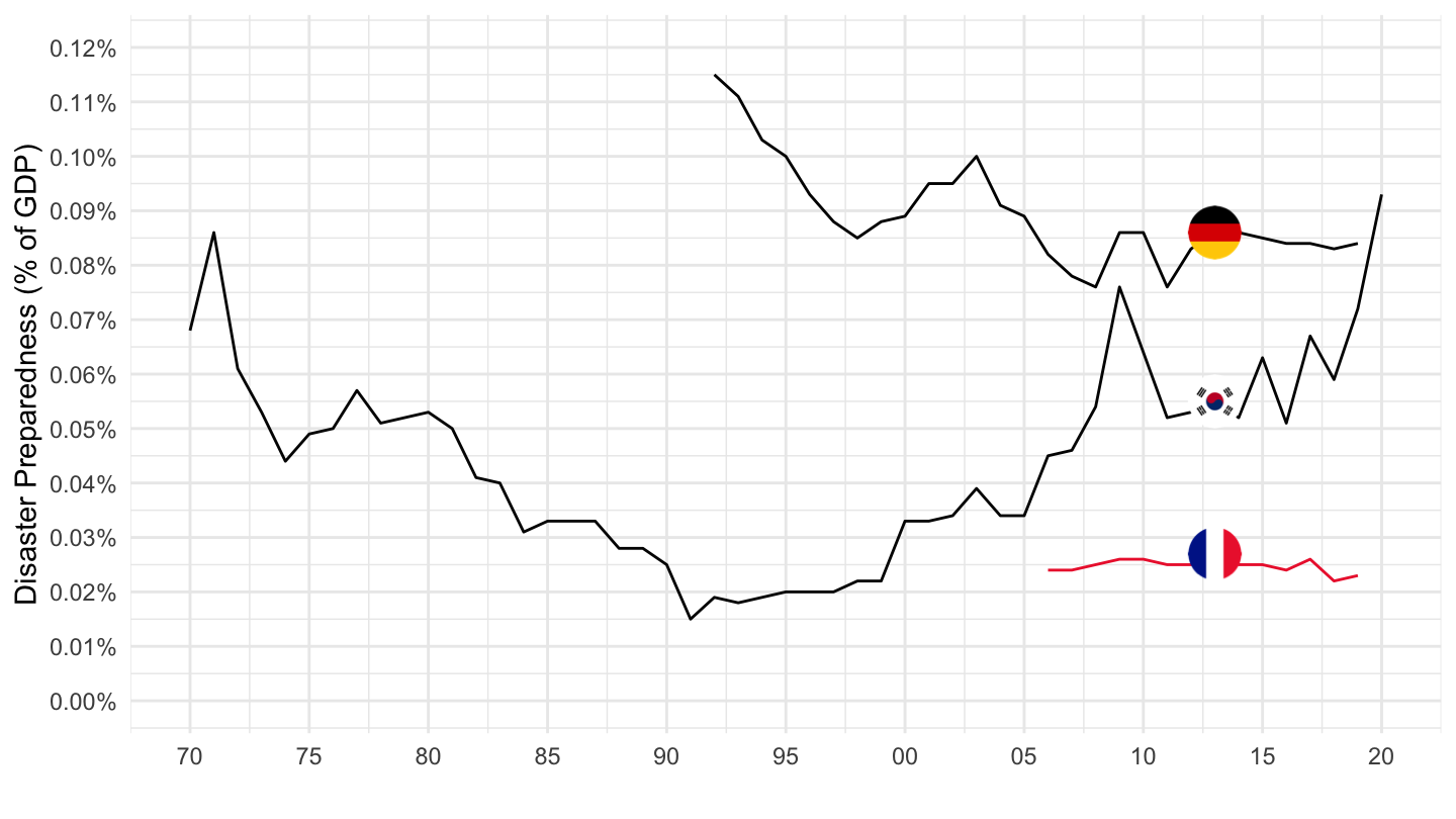
SHA |>
  filter(HC == "HC7",
         MEASURE == "PARPIB",
         HP == "HPTOT",
         HF == "HFTOT") |>
  left_join(SHA_var$LOCATION |>
              setNames(c("LOCATION", "Location")), by = "LOCATION") |>
  group_by(LOCATION, Location) |>
  summarise(Nobs = n(),
            `Year 1` = first(obsTime),
            `Administration 1 (% of GDP)` = first(obsValue),
            `Year 2` = last(obsTime),
            `Administration 2 (% of GDP)` = last(obsValue)) |>
  arrange(-`Administration 2 (% of GDP)`) |>
print_table_conditional()SHA |>
filter(HC == "HC7",
MEASURE == "PARPIB",
HP == "HPTOT",
HF == "HFTOT",
LOCATION %in% c("FRA", "DEU", "KOR")) |>
left_join(SHA_var$LOCATION, by = "LOCATION") |>
year_to_date() |>
add_flag_color("Location") |>
mutate(obsValue = obsValue/100) |>
ggplot() + geom_line(aes(x = date, y = obsValue, color = color)) +
scale_color_identity() + theme_minimal() + add_3flags +
scale_x_date(breaks = seq(1920, 2100, 5) |> paste0("-01-01") |> as.Date(),
labels = date_format("%Y")) +
scale_y_continuous(breaks = 0.01*seq(-7, 60, 0.05),
labels = scales::percent_format(accuracy = 0.01)) +
ylab("Administration (% of GDP)") + xlab("")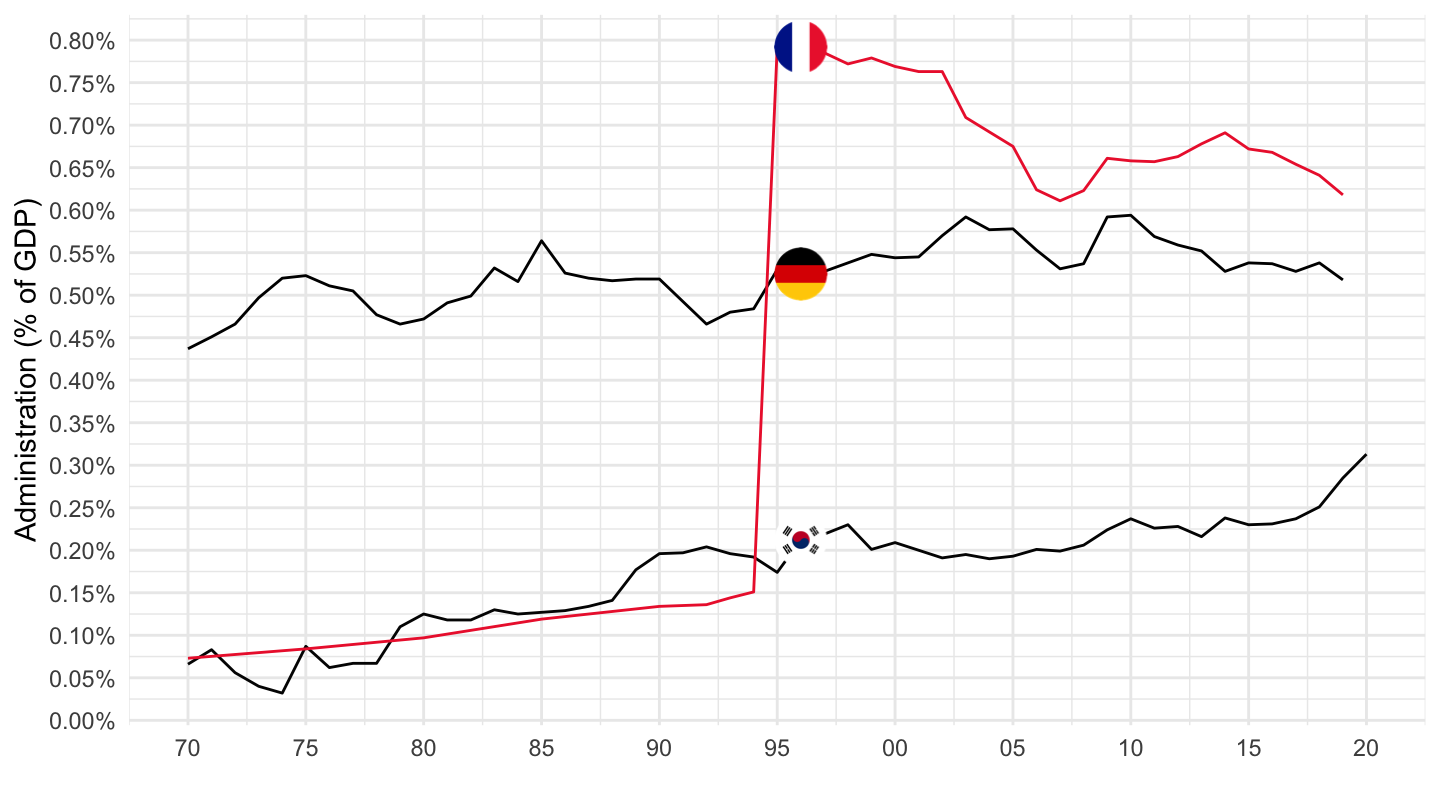
SHA |>
  filter(HC == "HC72",
         MEASURE == "PARPIB",
         HP == "HPTOT",
         HF == "HFTOT") |>
  left_join(SHA_var$LOCATION, by = "LOCATION") |>
  group_by(LOCATION, Location) |>
  summarise(Nobs = n(),
            `Year 1` = first(obsTime),
            `Administration 1 (% of GDP)` = first(obsValue),
            `Year 2` = last(obsTime),
            `Administration 2 (% of GDP)` = last(obsValue)) |>
  arrange(-`Administration 2 (% of GDP)`) |>
print_table_conditional()SHA |>
filter(HC == "HC72",
MEASURE == "PARPIB",
HP == "HPTOT",
HF == "HFTOT",
LOCATION %in% c("FRA", "DEU", "KOR")) |>
left_join(SHA_var$LOCATION, by = "LOCATION") |>
year_to_date() |>
add_flag_color("Location") |>
mutate(obsValue = obsValue/100) |>
ggplot() + geom_line(aes(x = date, y = obsValue, color = color)) +
scale_color_identity() + theme_minimal() + add_3flags +
scale_x_date(breaks = seq(1920, 2100, 5) |> paste0("-01-01") |> as.Date(),
labels = date_format("%Y")) +
scale_y_continuous(breaks = 0.01*seq(-7, 60, 0.05),
labels = scales::percent_format(accuracy = 0.01)) +
ylab("Administration (% of GDP)") + xlab("")