Info

LAST_DOWNLOAD

tibble(LAST_DOWNLOAD = as.Date(file.info("~/Dropbox/website/data/oecd/MEI_BOP6.RData")$mtime)) %>%
  print_table_conditional()

LAST_DOWNLOAD
2024-04-17

LAST_COMPILE

LAST_COMPILE
2024-04-17

Last

obsTime	Nobs
2023-Q4	7

Layout - By country

OECD Website. html

Nobs - Javascript

MEI_BOP6 %>%
  left_join(MEI_BOP6_var$SUBJECT, by = "SUBJECT") %>%
  {if (!is_html_output()) mutate(., Subject = substr(Subject, 1, 87)) else .} %>%
  group_by(SUBJECT, Subject, MEASURE, FREQUENCY) %>%
  filter(!is.na(obsValue)) %>%
  summarise(Nobs = n()) %>%
  arrange(-Nobs) %>%
  print_table_conditional

SUBJECT

All

MEI_BOP6 %>%
  left_join(MEI_BOP6_var$SUBJECT, by = "SUBJECT") %>%
  group_by(SUBJECT, Subject) %>%
  summarise(Nobs = n()) %>%
  arrange(-Nobs) %>%
  print_table_conditional

China

MEI_BOP6 %>%
  filter(LOCATION == "CHN") %>%
  left_join(MEI_BOP6_var$SUBJECT, by = "SUBJECT") %>%
  group_by(SUBJECT, Subject) %>%
  summarise(Nobs = n()) %>%
  arrange(-Nobs) %>%
  print_table_conditional

MEASURE

MEI_BOP6 %>%
  left_join(MEI_BOP6_var$MEASURE, by = "MEASURE") %>%
  group_by(MEASURE, Measure) %>%
  summarise(Nobs = n()) %>%
  arrange(-Nobs) %>%
  print_table_conditional

MEASURE	Measure	Nobs
CXCU	US-Dollar converted	297144
NCCU	National Currency	212319
CXCUSA	US-Dollar converted, Seasonally adjusted	120273
NCCUSA	National Currency, Seasonally adjusted	86970
STSA	Indicators in percentage	36472

FREQUENCY

MEI_BOP6 %>%
  left_join(MEI_BOP6_var$FREQUENCY, by = "FREQUENCY") %>%
  group_by(FREQUENCY, Frequency) %>%
  summarise(Nobs = n()) %>%
  arrange(-Nobs) %>%
  print_table_conditional

FREQUENCY	Frequency	Nobs
Q	Quarterly	581909
A	Annual	141869
M	Monthly	29400

LOCATION

MEI_BOP6 %>%
  left_join(MEI_BOP6_var$LOCATION, by = "LOCATION") %>%
  group_by(LOCATION, Location) %>%
  summarise(Nobs = n()) %>%
  arrange(-Nobs) %>%
  mutate(Flag = gsub(" ", "-", str_to_lower(Location)),
         Flag = paste0('<img src="../../icon/flag/vsmall/', Flag, '.png" alt="Flag">')) %>%
  select(Flag, everything()) %>%
  {if (is_html_output()) datatable(., filter = 'top', rownames = F, escape = F) else .}

obsTime

MEI_BOP6 %>%
  group_by(obsTime) %>%
  summarise(Nobs = n()) %>%
  arrange(desc(obsTime)) %>%
  print_table_conditional

Example

CA (% of GDP)

US, Europe, France, Germany

1990-

MEI_BOP6 %>%
  filter(SUBJECT == "B6BLTT02", 
         LOCATION %in% c("FRA", "DEU", "USA", "EA20"),
         FREQUENCY == "Q") %>%
  left_join(MEI_BOP6_var$LOCATION, by = "LOCATION") %>%
  quarter_to_date %>%
  filter(year(date) >= 1990) %>%
  mutate(obsValue = obsValue / 100) %>%
  ggplot() + ylab("Current Account (% of GDP)") + xlab("") + theme_minimal() +
  geom_line(aes(x = date, y = obsValue, color = Location, linetype = Location)) +
  scale_x_date(breaks = seq(1920, 2025, 2) %>% paste0("-01-01") %>% as.Date,
               labels = date_format("%Y")) +
  theme(legend.position = c(0.2, 0.9),
        legend.title = element_blank()) +
  scale_y_continuous(breaks = 0.01*seq(-7, 16, 1),
                     labels = scales::percent_format(accuracy = 1)) +
  geom_hline(yintercept = 0, linetype = "dashed", color = "black")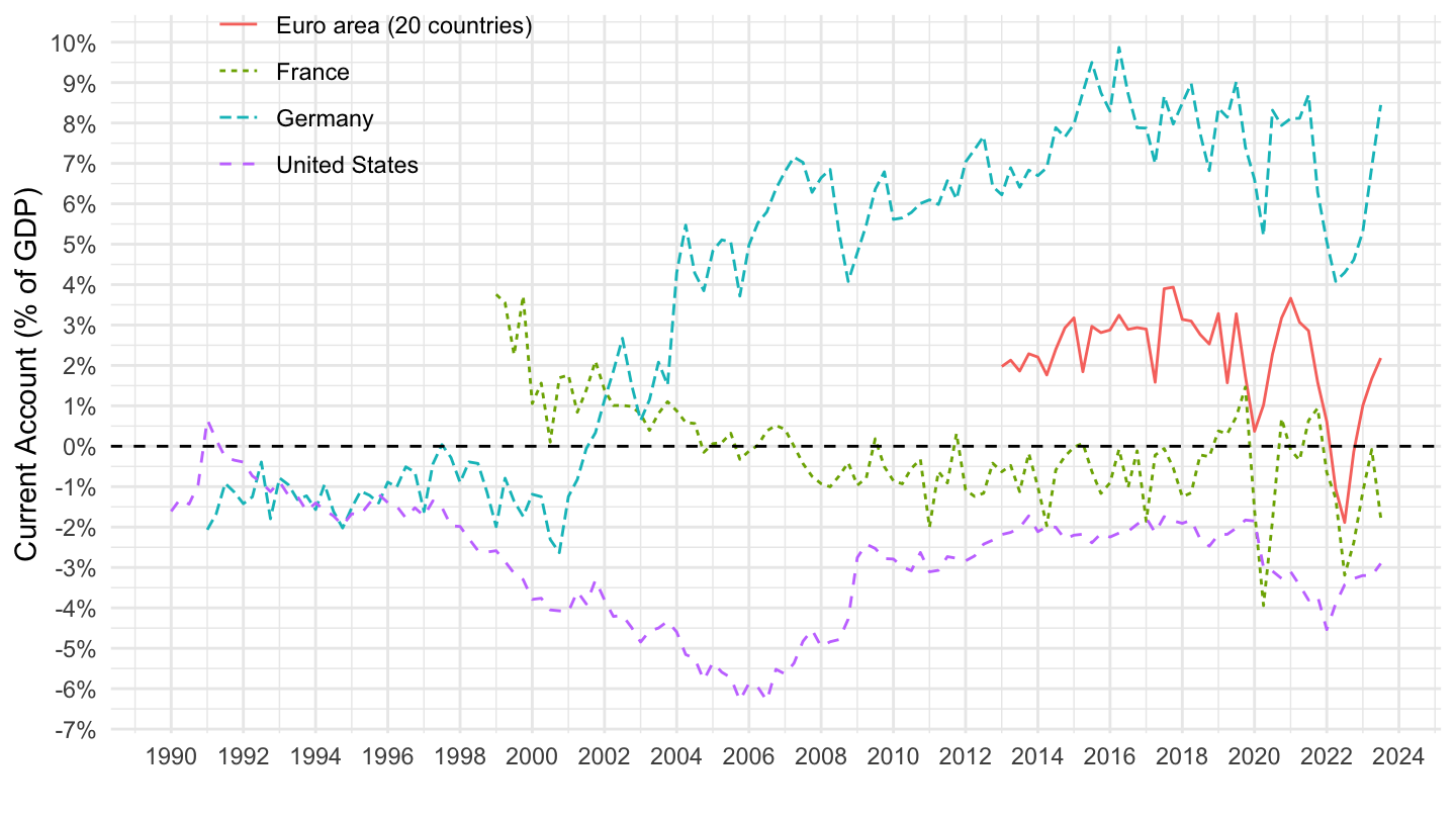

1999-

MEI_BOP6 %>%
  filter(SUBJECT == "B6BLTT02", 
         LOCATION %in% c("FRA", "DEU", "USA", "EA20"),
         FREQUENCY == "Q") %>%
  left_join(MEI_BOP6_var$LOCATION, by = "LOCATION") %>%
  quarter_to_date %>%
  filter(year(date) >= 1999) %>%
  mutate(obsValue = obsValue / 100) %>%
  mutate(Location = ifelse(LOCATION == "EA20", "Europe", Location)) %>%
  left_join(colors, by = c("Location" = "country")) %>%
  ggplot() + ylab("Current Account (% of GDP)") + xlab("") + theme_minimal() +
  geom_line(aes(x = date, y = obsValue, color = color)) +
  scale_x_date(breaks = seq(1920, 2025, 2) %>% paste0("-01-01") %>% as.Date,
               labels = date_format("%Y")) +
  theme(legend.position = c(0.2, 0.9),
        legend.title = element_blank()) +
  scale_color_identity() + add_4flags +
  scale_y_continuous(breaks = 0.01*seq(-7, 16, 1),
                     labels = scales::percent_format(accuracy = 1)) +
  geom_hline(yintercept = 0, linetype = "dashed", color = "black")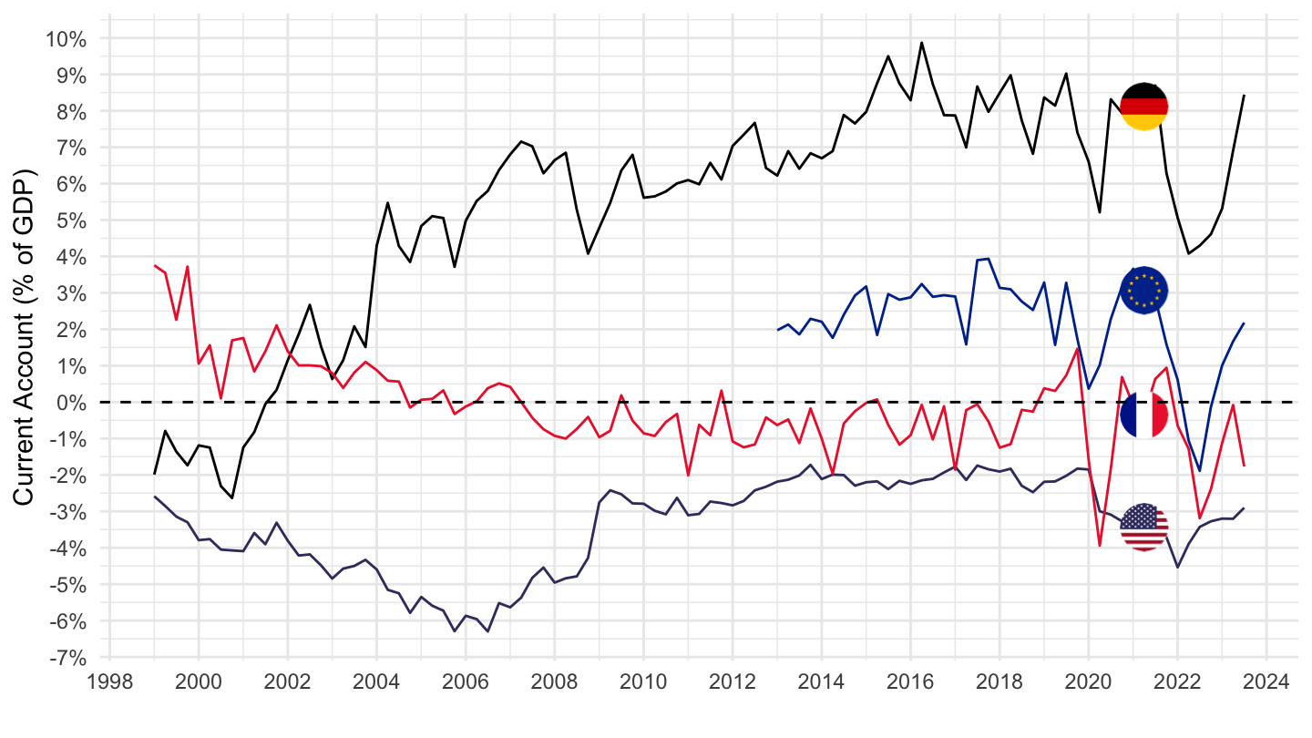

Belgium, Greece, Netherlands

Annual

MEI_BOP6 %>%
  filter(SUBJECT == "B6BLTT02", 
         LOCATION %in% c("BEL", "GRC", "NLD"),
         FREQUENCY == "A") %>%
  left_join(MEI_BOP6_var$LOCATION, by = "LOCATION") %>%
  year_to_date %>%
  filter(year(date) >= 1990) %>%
  ggplot() + ylab("Current Account (% of GDP)") + xlab("") + theme_minimal() +
  geom_line(aes(x = date, y = obsValue / 100, color = Location, linetype = Location)) +
  scale_color_manual(values = viridis(4)[1:3]) +
  scale_x_date(breaks = seq(1920, 2025, 2) %>% paste0("-01-01") %>% as.Date,
               labels = date_format("%Y")) +
  theme(legend.position = c(0.2, 0.9),
        legend.title = element_blank()) +
  scale_y_continuous(breaks = 0.01*seq(-7, 16, 1),
                     labels = scales::percent_format(accuracy = 1)) +
  geom_hline(yintercept = 0, linetype = "dashed", color = "black")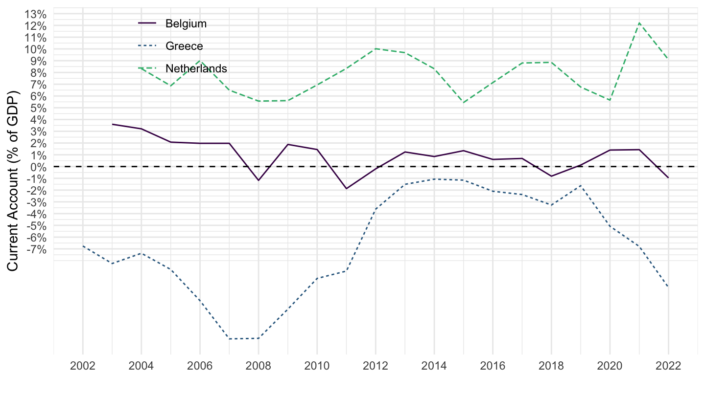

France and Germany

Annual

MEI_BOP6 %>%
  filter(SUBJECT == "B6BLTT02", 
         LOCATION %in% c("FRA", "DEU"),
         FREQUENCY == "A") %>%
  left_join(MEI_BOP6_var$LOCATION, by = "LOCATION") %>%
  year_to_date %>%
  filter(year(date) >= 1990) %>%
  ggplot() + ylab("Current Account (% of GDP)") + xlab("") + theme_minimal() +
  geom_line(aes(x = date, y = obsValue / 100, color = Location, linetype = Location)) +
  scale_color_manual(values = viridis(3)[1:2]) +
  scale_x_date(breaks = seq(1920, 2025, 2) %>% paste0("-01-01") %>% as.Date,
               labels = date_format("%Y")) +
  theme(legend.position = c(0.2, 0.9),
        legend.title = element_blank()) +
  scale_y_continuous(breaks = 0.01*seq(-7, 16, 1),
                     labels = scales::percent_format(accuracy = 1)) +
  geom_hline(yintercept = 0, linetype = "dashed", color = "black")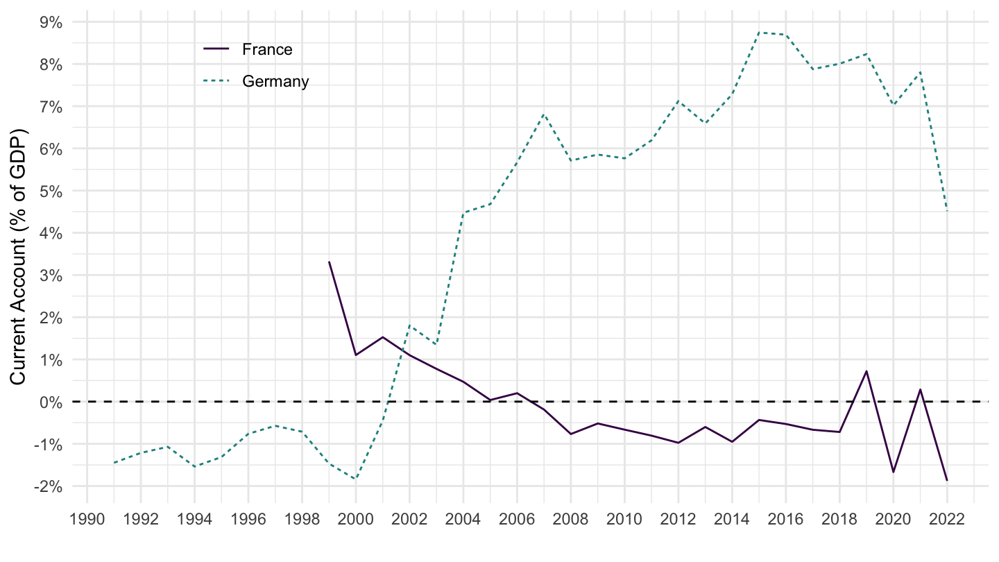

Quarterly

MEI_BOP6 %>%
  filter(SUBJECT == "B6BLTT02", 
         LOCATION %in% c("FRA", "DEU"),
         FREQUENCY == "Q") %>%
  left_join(MEI_BOP6_var$LOCATION, by = "LOCATION") %>%
  quarter_to_date %>%
  filter(year(date) >= 1990) %>%
  ggplot() + ylab("Current Account (% of GDP)") + xlab("") + theme_minimal() +
  geom_line(aes(x = date, y = obsValue / 100, color = Location, linetype = Location)) +
  scale_color_manual(values = viridis(3)[1:2]) +
  scale_x_date(breaks = seq(1920, 2025, 2) %>% paste0("-01-01") %>% as.Date,
               labels = date_format("%Y")) +
  theme(legend.position = c(0.2, 0.9),
        legend.title = element_blank()) +
  scale_y_continuous(breaks = 0.01*seq(-7, 16, 1),
                     labels = scales::percent_format(accuracy = 1)) +
  geom_hline(yintercept = 0, linetype = "dashed", color = "black")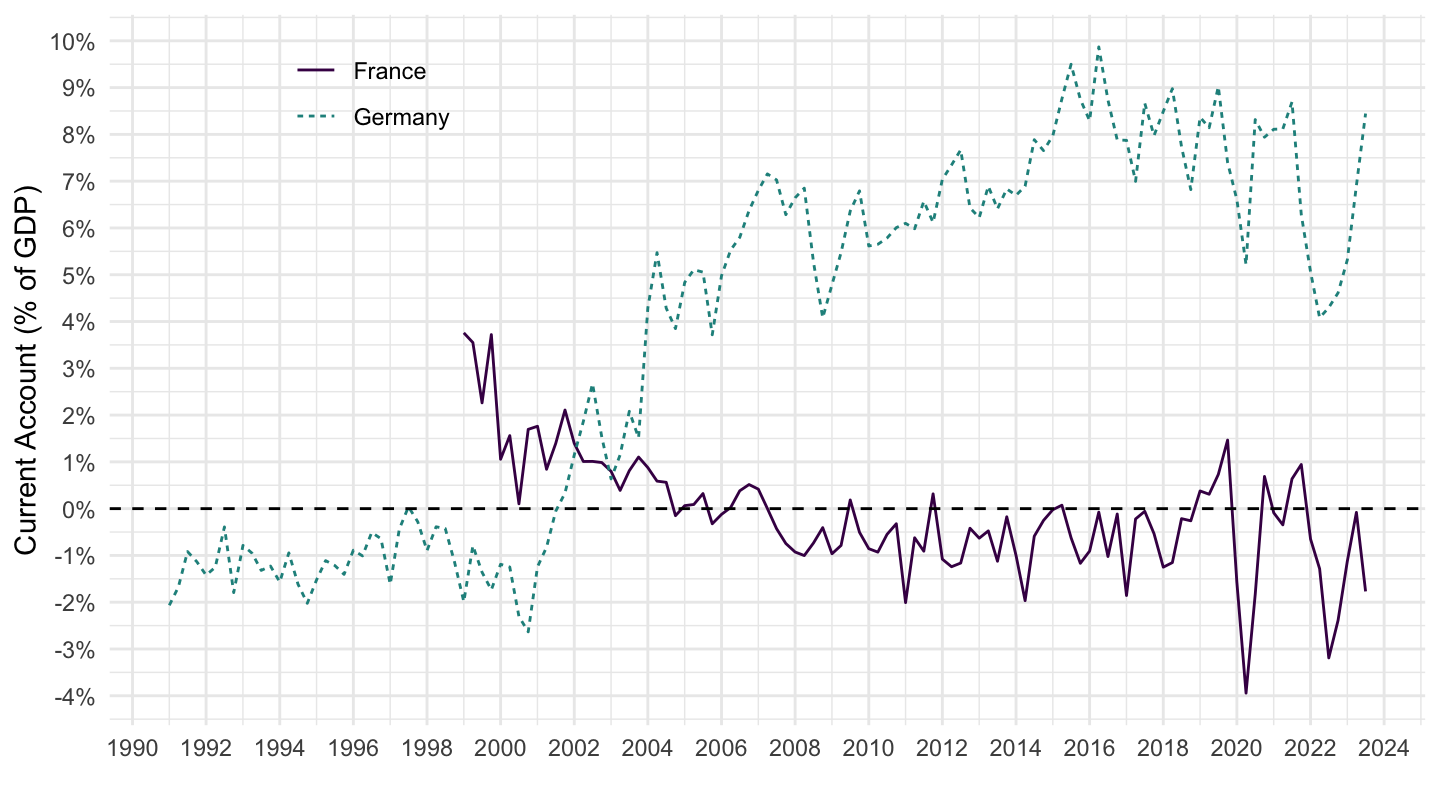

Netherlands, Denmark, Italy

MEI_BOP6 %>%
  filter(SUBJECT == "B6BLTT02", 
         LOCATION %in% c("NLD", "DNK", "ITA"),
         FREQUENCY == "A") %>%
  left_join(MEI_BOP6_var$LOCATION, by = "LOCATION") %>%
  year_to_date %>%
  filter(year(date) >= 1990) %>%
  ggplot() + ylab("Current Account (% of GDP)") + xlab("") + theme_minimal() +
  geom_line(aes(x = date, y = obsValue/100, color = Location, linetype = Location)) +
  scale_color_manual(values = viridis(4)[1:3]) +
  scale_x_date(breaks = seq(1920, 2025, 2) %>% paste0("-01-01") %>% as.Date,
               labels = date_format("%Y")) +
  theme(legend.position = c(0.2, 0.9),
        legend.title = element_blank()) +
  scale_y_continuous(breaks = 0.01*seq(-7, 16, 1),
                     labels = scales::percent_format(accuracy = 1)) +
  geom_hline(yintercept = 0, linetype = "dashed", color = "black")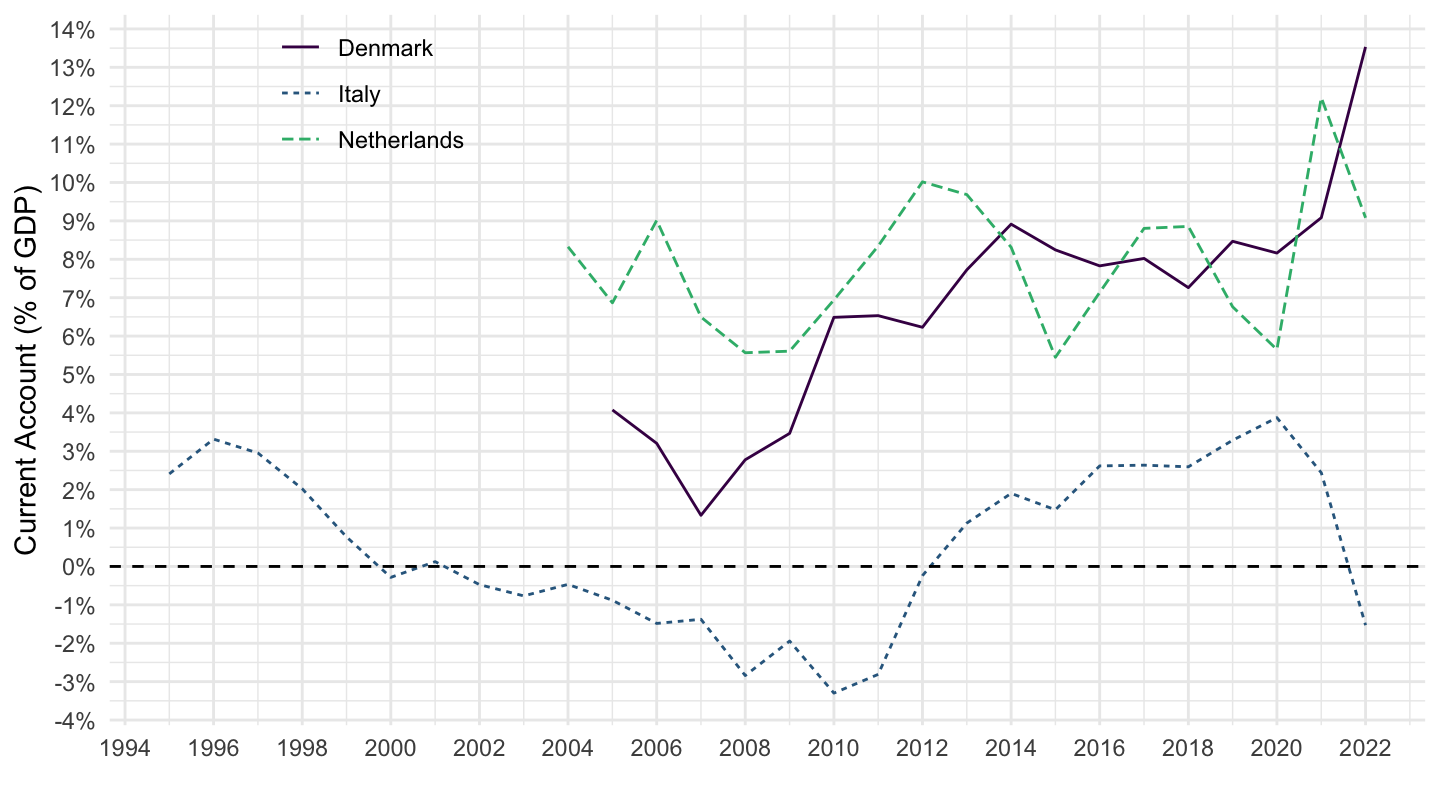

Australia, Japan, Switzerland

MEI_BOP6 %>%
  filter(SUBJECT == "B6BLTT02", 
         LOCATION %in% c("AUS", "CHE", "JPN"),
         FREQUENCY == "A") %>%
  left_join(MEI_BOP6_var$LOCATION, by = "LOCATION") %>%
  year_to_date %>%
  filter(year(date) >= 1990) %>%
  ggplot() + ylab("Current Account (% of GDP)") + xlab("") + theme_minimal() +
  geom_line(aes(x = date, y = obsValue/100, color = Location, linetype = Location)) +
  scale_color_manual(values = viridis(4)[1:3]) +
  scale_x_date(breaks = seq(1920, 2025, 2) %>% paste0("-01-01") %>% as.Date,
               labels = date_format("%Y")) +
  theme(legend.position = c(0.2, 0.9),
        legend.title = element_blank()) +
  scale_y_continuous(breaks = 0.01*seq(-7, 16, 1),
                     labels = scales::percent_format(accuracy = 1)) +
  geom_hline(yintercept = 0, linetype = "dashed", color = "black")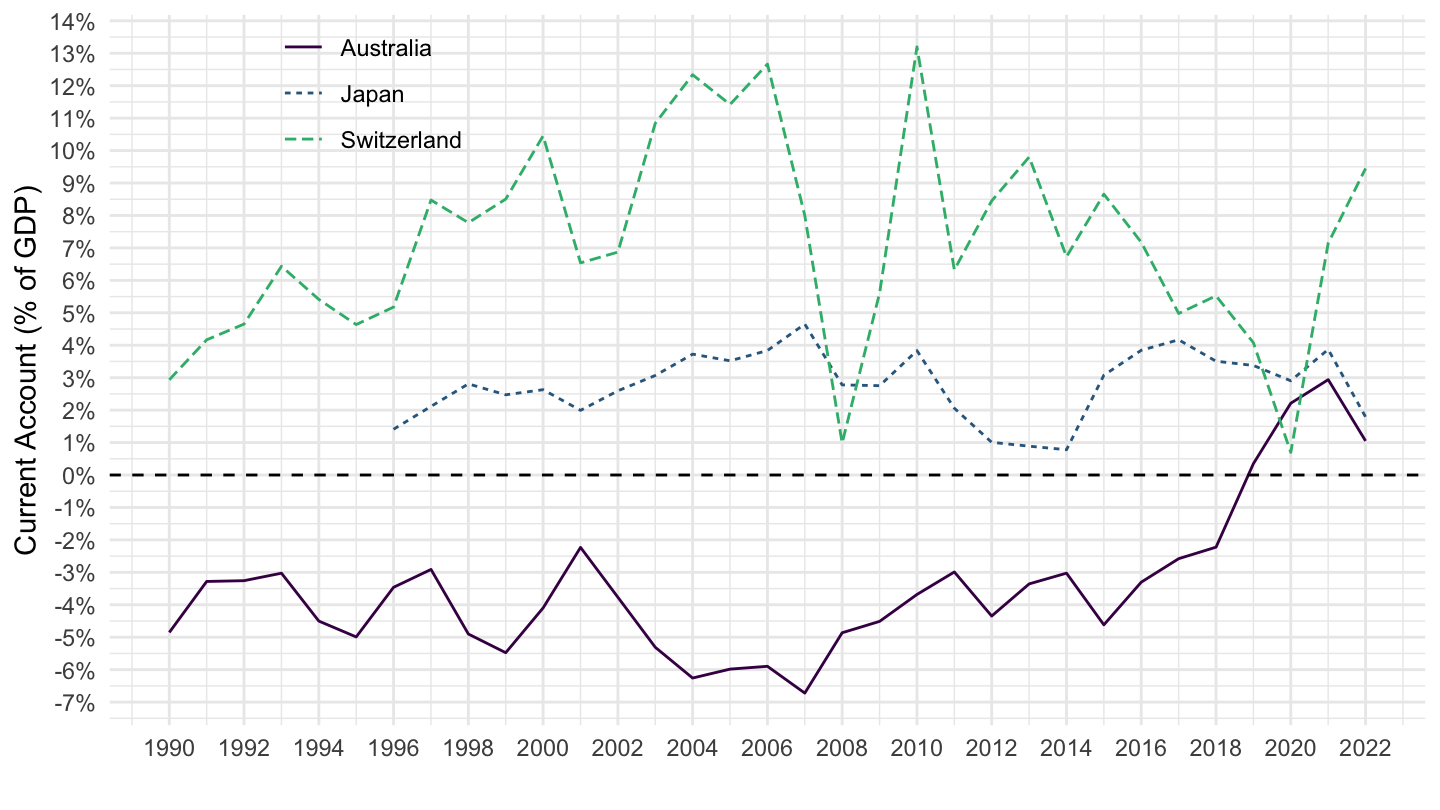

Current Account Balance

France, Germany, Italy

MEI_BOP6 %>%
  filter(LOCATION %in% c("FRA", "DEU", "ITA"),
         # B6BLTT01: Balance of payments BPM6 > Current account Balance > Total > Total Balance
         SUBJECT == "B6BLTT01",
         # CXCUSA: US Dollars, sum over component sub-periods, s.a
         MEASURE == "CXCUSA",
         FREQUENCY == "Q") %>%
  quarter_to_date %>%
  left_join(MEI_BOP6_var$LOCATION, by = "LOCATION") %>%
  group_by(LOCATION) %>%
  ggplot(.) + 
  geom_line(aes(x = date, y = obsValue/10^3, color = Location, linetype = Location)) + 
  theme_minimal() + scale_color_manual(values = viridis(4)[1:3]) +
  theme(legend.title = element_blank(),
        legend.position = c(0.2, 0.8)) +
  scale_x_date(breaks = seq(1950, 2100, 5) %>% paste0("-01-01") %>% as.Date,
               labels = date_format("%Y")) +
  scale_y_continuous(breaks = seq(-20000, 400000, 10),
                     labels = dollar_format(accuracy = 1, suffix = " Bn", prefix = "$ ")) + 
  xlab("") + ylab("Current account Balance, Total") +
  geom_hline(yintercept = 0, linetype = "dashed", color = "black")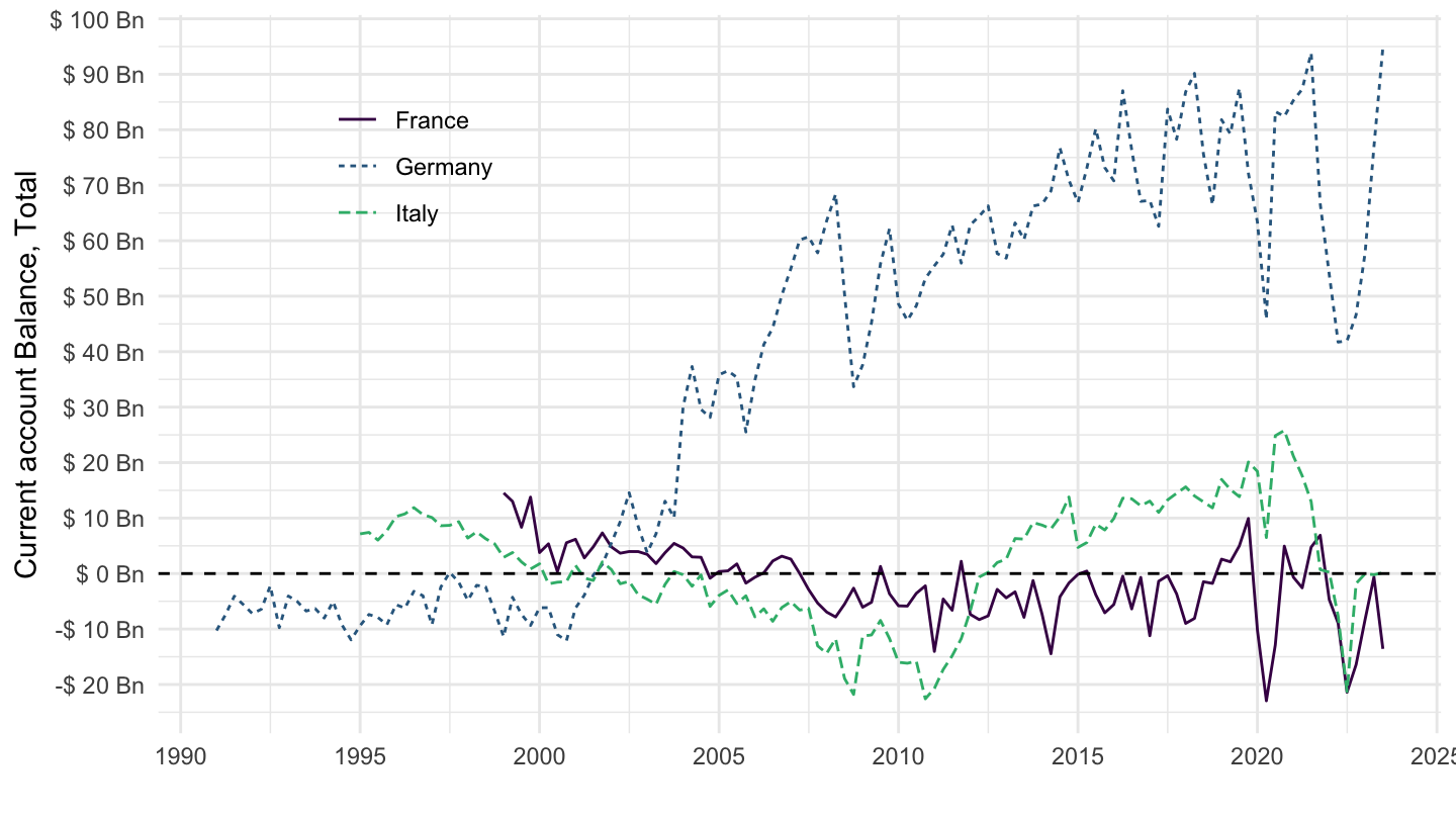

Netherlands, Switzerland, Sweden

MEI_BOP6 %>%
  filter(LOCATION %in% c("NLD", "SWE", "CHE"),
         # B6BLTT01: Balance of payments BPM6 > Current account Balance > Total > Total Balance
         SUBJECT == "B6BLTT01",
         # CXCUSA: US Dollars, sum over component sub-periods, s.a
         MEASURE == "CXCUSA",
         FREQUENCY == "Q") %>%
  quarter_to_date %>%
  left_join(MEI_BOP6_var$LOCATION, by = "LOCATION") %>%
  group_by(LOCATION) %>%
  ggplot(.) + 
  geom_line(aes(x = date, y = obsValue/10^3, color = Location, linetype = Location)) + 
  theme_minimal() + scale_color_manual(values = viridis(4)[1:3]) +
  theme(legend.title = element_blank(),
        legend.position = c(0.2, 0.8)) +
  scale_x_date(breaks = seq(1950, 2100, 5) %>% paste0("-01-01") %>% as.Date,
               labels = date_format("%Y")) +
  scale_y_continuous(breaks = seq(-20000, 400000, 10),
                     labels = dollar_format(accuracy = 1, suffix = " Bn", prefix = "$ ")) + 
  xlab("") + ylab("Current account Balance, Total") +
  geom_hline(yintercept = 0, linetype = "dashed", color = "black")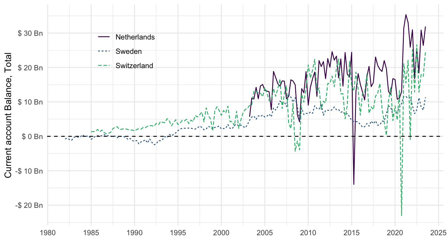

CA Decompositions - ALL

Goods and Services Account. IMF
Primary Income. IMF
Secondary Income. IMF

Germany

MEI_BOP6 %>%
  filter(LOCATION %in% c("DEU"),
         # B6BLTT01: Current account, balance
         # B6BLPI01: Primary income, balance
         # B6BLSI01: Secondary income, balance
         SUBJECT %in% c("B6BLTT01", "B6BLPI01", "B6BLSI01", "B6BLTD01", "B6BLSE01"),
         # CXCUSA: US Dollars, sum over component sub-periods, s.a
         MEASURE == "CXCUSA",
         FREQUENCY == "Q") %>%
  quarter_to_date %>%
  left_join(MEI_BOP6_var$SUBJECT, by = "SUBJECT") %>%
  group_by(LOCATION) %>%
  ggplot(.) + xlab("") + ylab("Current account Balance Component, Total") + 
  geom_line(aes(x = date, y = obsValue/10^3, color = Subject)) + 
  theme_minimal() + scale_color_manual(values = viridis(6)[1:5]) +
  theme(legend.title = element_blank(),
        legend.position = c(0.2, 0.8),
        legend.text = element_text(size = 8),
        legend.key.size = unit(0.9, 'lines')) +
  scale_x_date(breaks = seq(1950, 2100, 5) %>% paste0("-01-01") %>% as.Date,
               labels = date_format("%Y")) +
  scale_y_continuous(breaks = seq(-20000, 400000, 10),
                     labels = dollar_format(accuracy = 1, suffix = " Bn", prefix = "$ ")) +
  geom_hline(yintercept = 0, linetype = "dashed", color = "black")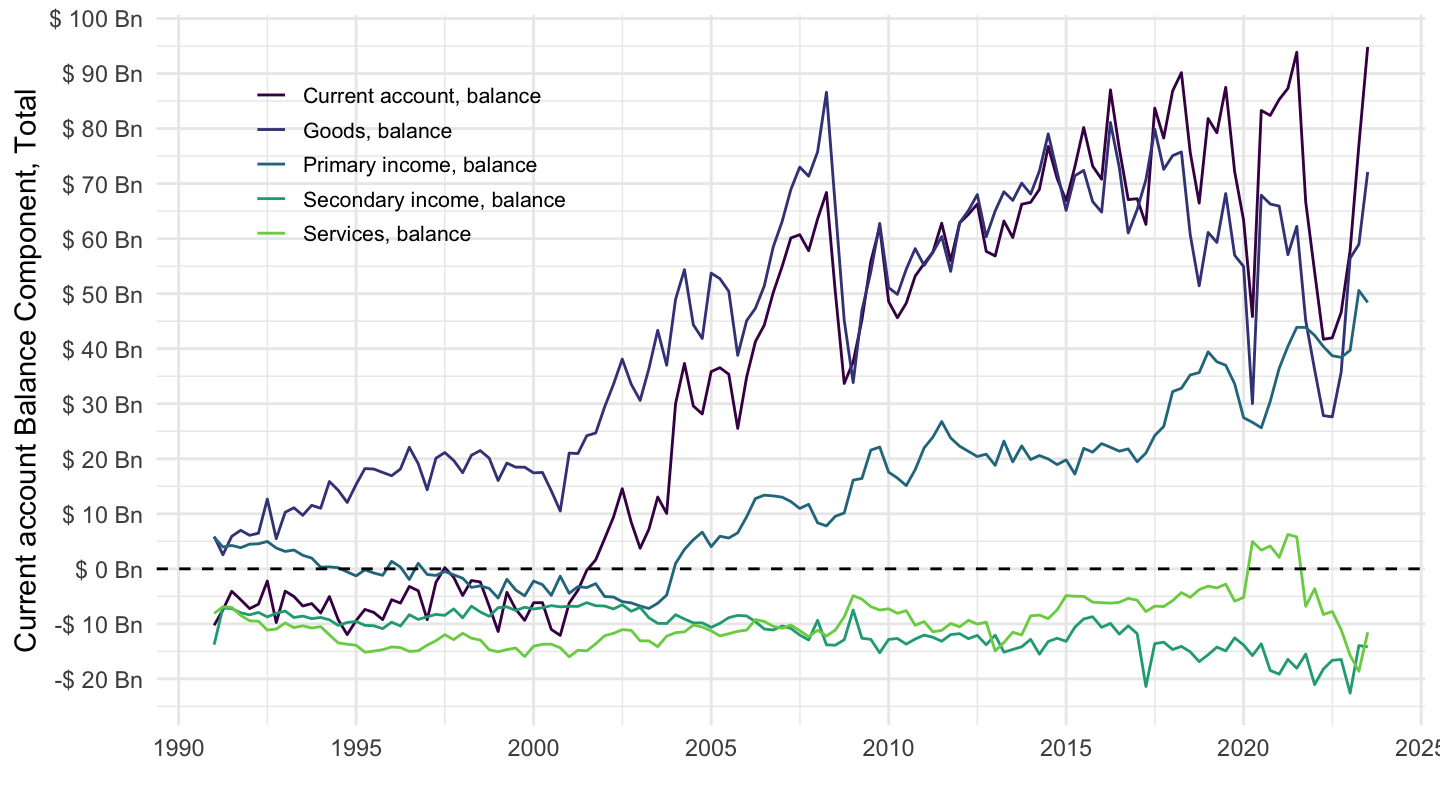

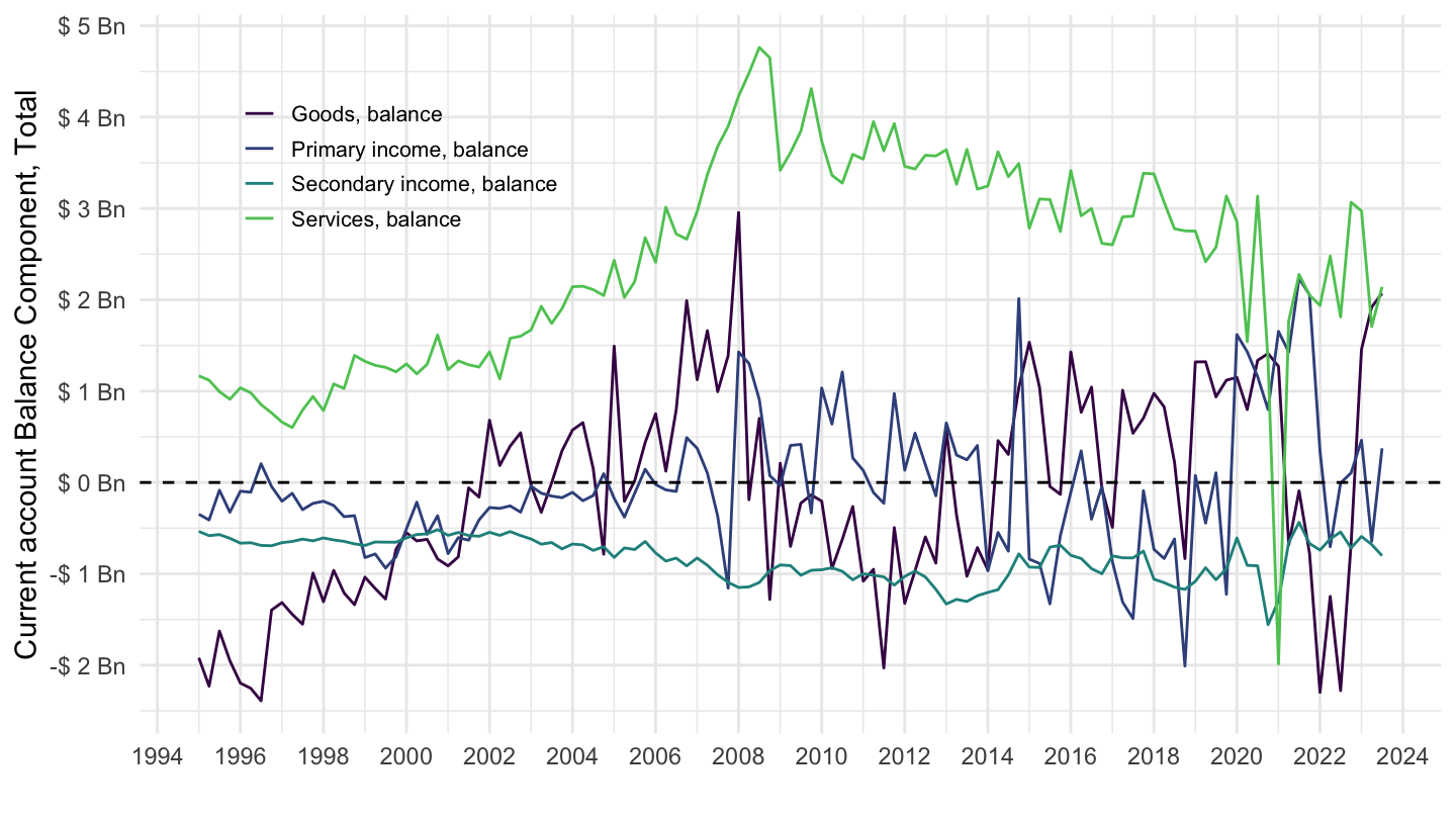
France

MEI_BOP6 %>%
  filter(LOCATION %in% c("FRA"),
         # B6BLTT01: Current account, balance
         # B6BLPI01: Primary income, balance
         # B6BLSI01: Secondary income, balance
         SUBJECT %in% c("B6BLTT01", "B6BLPI01", "B6BLSI01", "B6BLTD01", "B6BLSE01"),
         # CXCUSA: US Dollars, sum over component sub-periods, s.a
         MEASURE == "CXCUSA",
         FREQUENCY == "Q") %>%
  quarter_to_date %>%
  left_join(MEI_BOP6_var$SUBJECT, by = "SUBJECT") %>%
  group_by(LOCATION) %>%
  ggplot(.) + xlab("") + ylab("Current account Balance Component, Total") + 
  geom_line(aes(x = date, y = obsValue/10^3, color = Subject)) + 
  theme_minimal() + scale_color_manual(values = viridis(6)[1:5]) +
  theme(legend.title = element_blank(),
        legend.position = c(0.2, 0.15),
        legend.text = element_text(size = 8),
        legend.key.size = unit(0.9, 'lines')) +
  scale_x_date(breaks = seq(1950, 2100, 5) %>% paste0("-01-01") %>% as.Date,
               labels = date_format("%Y")) +
  scale_y_continuous(breaks = seq(-20000, 400000, 10),
                     labels = dollar_format(accuracy = 1, suffix = " Bn", prefix = "$ ")) +
  geom_hline(yintercept = 0, linetype = "dashed", color = "black")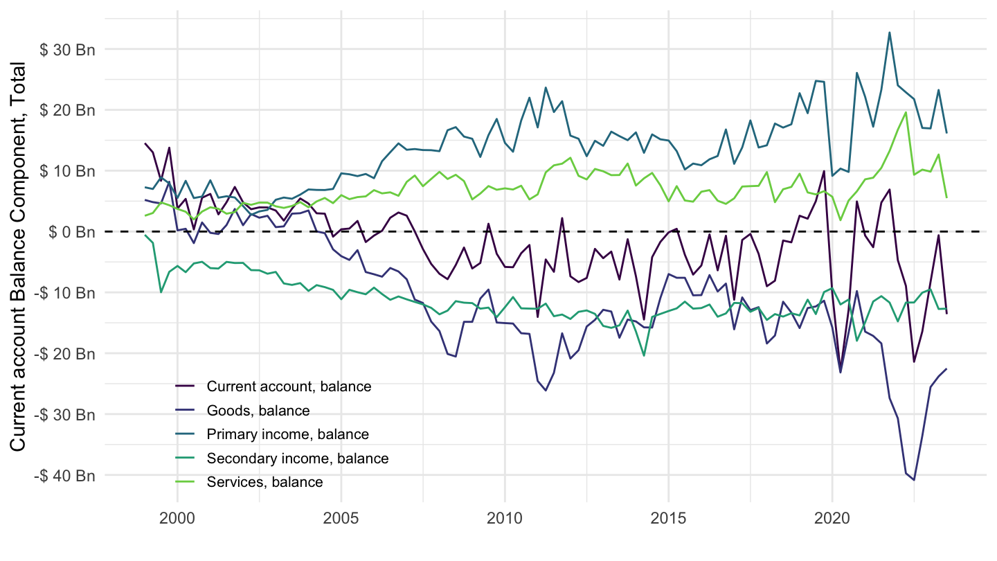

United States

MEI_BOP6 %>%
  filter(LOCATION %in% c("USA"),
         # B6BLTT01: Current account, balance
         # B6BLPI01: Primary income, balance
         # B6BLSI01: Secondary income, balance
         SUBJECT %in% c("B6BLTT01", "B6BLPI01", "B6BLSI01", "B6BLTD01", "B6BLSE01"),
         # CXCUSA: US Dollars, sum over component sub-periods, s.a
         MEASURE == "CXCUSA",
         FREQUENCY == "Q") %>%
  quarter_to_date %>%
  left_join(MEI_BOP6_var$SUBJECT, by = "SUBJECT") %>%
  group_by(LOCATION) %>%
  ggplot(.) + xlab("") + ylab("Current account Balance Component, Total") + 
  geom_line(aes(x = date, y = obsValue/10^3, color = Subject)) + 
  theme_minimal() + scale_color_manual(values = viridis(6)[1:5]) +
  theme(legend.title = element_blank(),
        legend.position = c(0.2, 0.2),
        legend.text = element_text(size = 8),
        legend.key.size = unit(0.9, 'lines')) +
  scale_x_date(breaks = seq(1950, 2100, 5) %>% paste0("-01-01") %>% as.Date,
               labels = date_format("%Y")) +
  scale_y_continuous(breaks = seq(-20000, 400000, 50),
                     labels = dollar_format(accuracy = 1, suffix = " Bn", prefix = "$ ")) +
  geom_hline(yintercept = 0, linetype = "dashed", color = "black")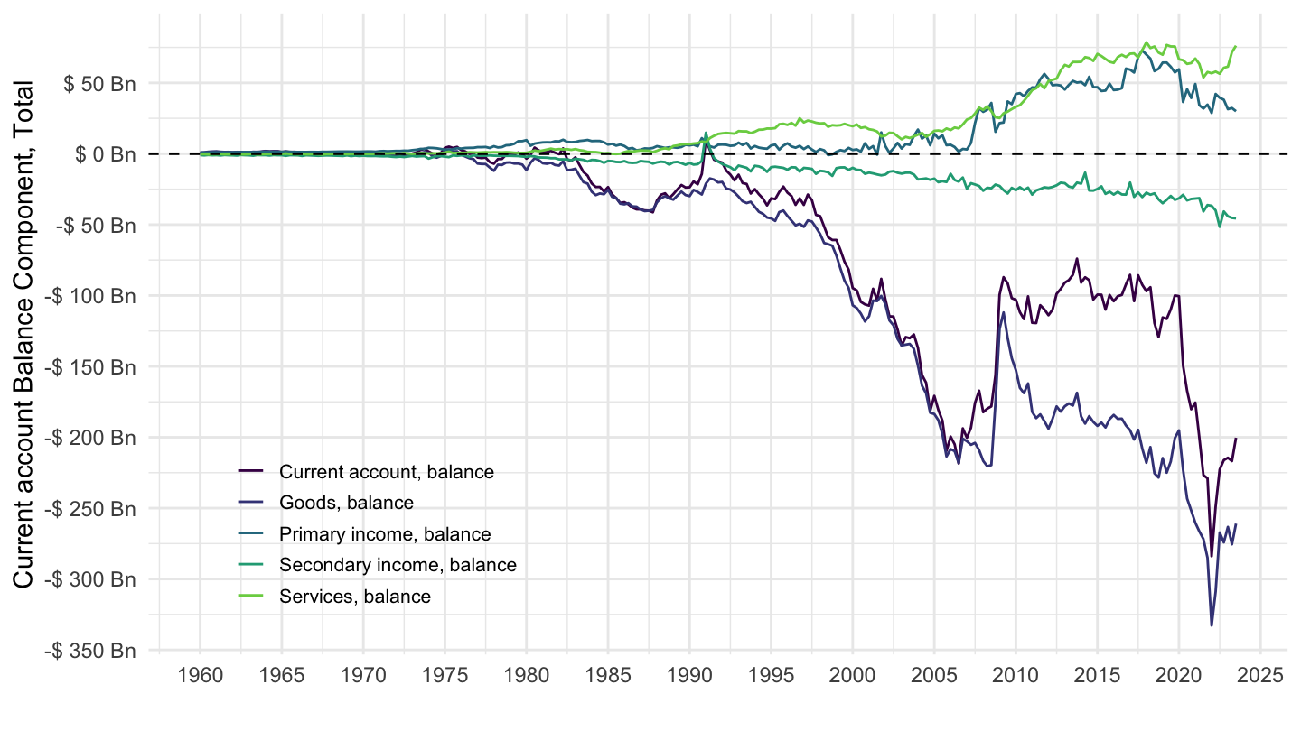

Capital Account Decompositions

Germany

MEI_BOP6 %>%
  filter(LOCATION %in% c("DEU"),
         # B6FADI01: Current account, balance
         # B6BLPI01: Primary income, balance
         # B6BLSI01: Secondary income, balance
         SUBJECT %in% c("B6FADI01", "B6FAPI10", "B6FAOI01", "B6FATT01"),
         MEASURE == "CXCU",
         # CXCUSA: US Dollars, sum over component sub-periods, s.a
         FREQUENCY == "Q") %>%
  quarter_to_date %>%
  left_join(MEI_BOP6_var$SUBJECT, by = "SUBJECT") %>%
  ggplot(.) + xlab("") + ylab("Current account Balance Component, Total") + 
  geom_line(aes(x = date, y = obsValue/10^3, color = Subject)) + 
  theme_minimal() + scale_color_manual(values = viridis(5)[1:4]) +
  theme(legend.title = element_blank(),
        legend.position = c(0.2, 0.8),
        legend.text = element_text(size = 8),
        legend.key.size = unit(0.9, 'lines')) +
  scale_x_date(breaks = seq(1950, 2100, 5) %>% paste0("-01-01") %>% as.Date,
               labels = date_format("%Y")) +
  scale_y_continuous(breaks = seq(-20000, 400000, 10),
                     labels = dollar_format(accuracy = 1, suffix = " Bn", prefix = "$ ")) +
  geom_hline(yintercept = 0, linetype = "dashed", color = "black")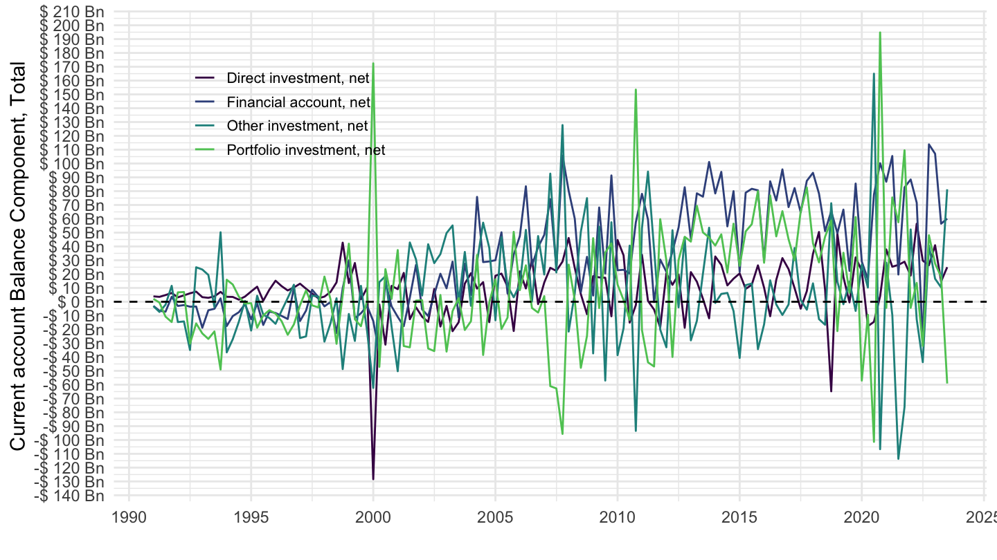

Euro Area

MEI_BOP6 %>%
  filter(LOCATION %in% c("EA20"),
         # B6BLTT01: Current account, balance
         # B6BLPI01: Primary income, balance
         # B6BLSI01: Secondary income, balance
         SUBJECT %in% c("B6FADI01", "B6FAPI10", "B6FAOI01", "B6FATT01"),
         # CXCU: US Dollars, sum over component sub-periods, s.a
         MEASURE == "CXCU",
         FREQUENCY == "Q") %>%
  quarter_to_date %>%
  left_join(MEI_BOP6_var$SUBJECT, by = "SUBJECT") %>%
  group_by(LOCATION) %>%
  ggplot(.) + xlab("") + ylab("Current account Balance Component, Total") + 
  geom_line(aes(x = date, y = obsValue/10^3, color = Subject)) + 
  theme_minimal() + scale_color_manual(values = viridis(5)[1:4]) +
  theme(legend.title = element_blank(),
        legend.position = c(0.2, 0.8),
        legend.text = element_text(size = 8),
        legend.key.size = unit(0.9, 'lines')) +
  scale_x_date(breaks = seq(1950, 2100, 2) %>% paste0("-01-01") %>% as.Date,
               labels = date_format("%Y")) +
  scale_y_continuous(breaks = seq(-20000, 400000, 20),
                     labels = dollar_format(accuracy = 1, suffix = " Bn", prefix = "$ ")) +
  geom_hline(yintercept = 0, linetype = "dashed", color = "black")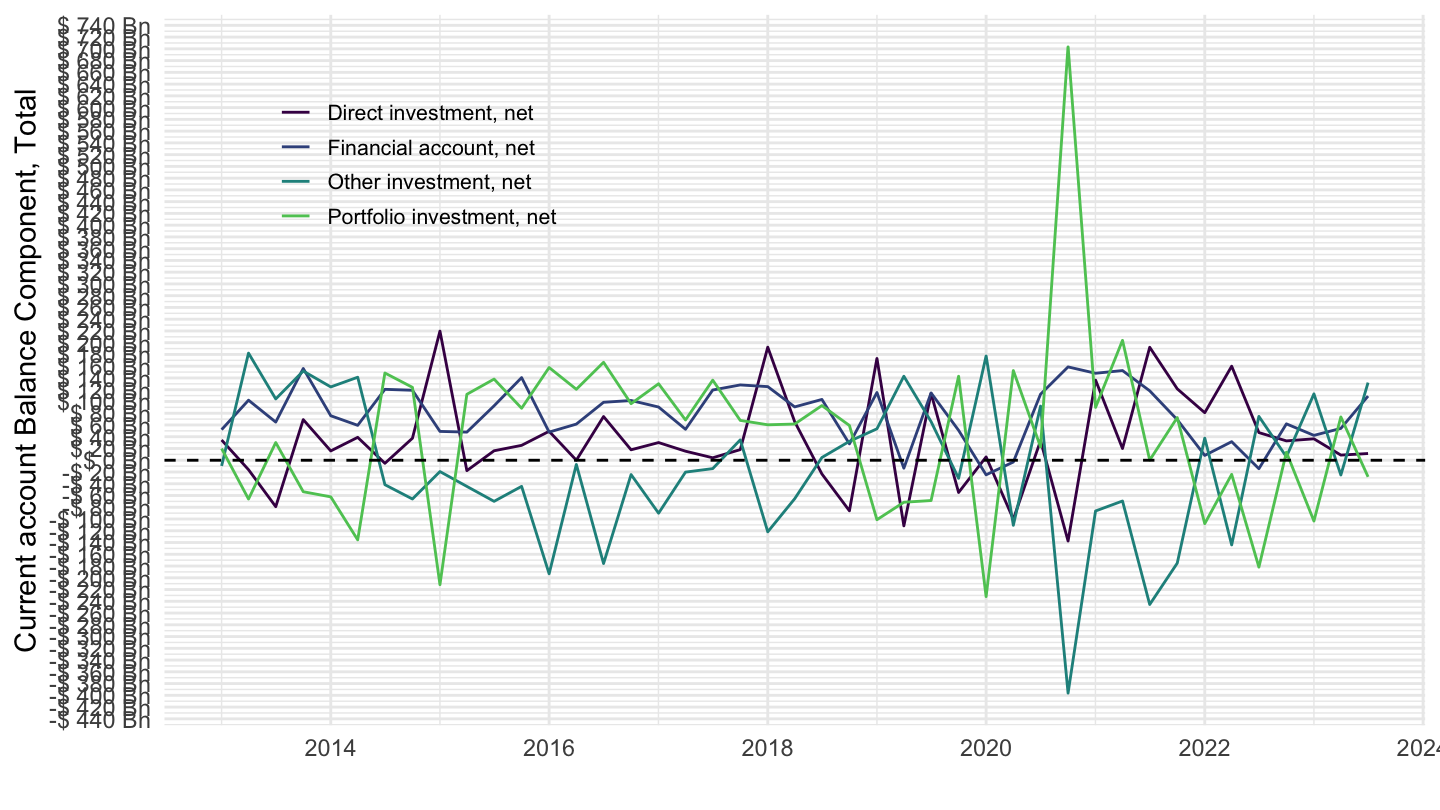

China

MEI_BOP6 %>%
  filter(LOCATION %in% c("CHN"),
         # B6BLTT01: Current account, balance
         # B6BLPI01: Primary income, balance
         # B6BLSI01: Secondary income, balance
         SUBJECT %in% c("B6FADI01", "B6FAPI10", "B6FAOI01", "B6FATT01"),
         # CXCU: US Dollars, sum over component sub-periods, s.a
         MEASURE == "CXCU",
         FREQUENCY == "Q") %>%
  quarter_to_date %>%
  left_join(MEI_BOP6_var$SUBJECT, by = "SUBJECT") %>%
  group_by(LOCATION) %>%
  ggplot(.) + xlab("") + ylab("Current account Balance Component, Total") + 
  geom_line(aes(x = date, y = obsValue/10^3, color = Subject)) + 
  theme_minimal() + scale_color_manual(values = viridis(5)[1:4]) +
  theme(legend.title = element_blank(),
        legend.position = c(0.2, 0.8),
        legend.text = element_text(size = 8),
        legend.key.size = unit(0.9, 'lines')) +
  scale_x_date(breaks = seq(1950, 2100, 5) %>% paste0("-01-01") %>% as.Date,
               labels = date_format("%Y")) +
  scale_y_continuous(breaks = seq(-20000, 400000, 50),
                     labels = dollar_format(accuracy = 1, suffix = " Bn", prefix = "$ ")) +
  geom_hline(yintercept = 0, linetype = "dashed", color = "black")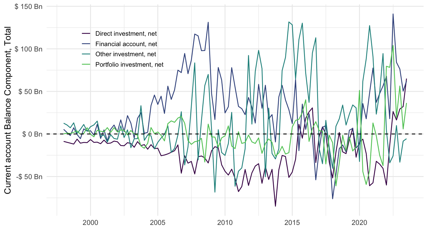

United Kingdom

MEI_BOP6 %>%
  filter(LOCATION %in% c("GBR"),
         # B6BLTT01: Current account, balance
         # B6BLPI01: Primary income, balance
         # B6BLSI01: Secondary income, balance
         SUBJECT %in% c("B6FADI01", "B6FAPI10", "B6FAOI01", "B6FATT01"),
         # CXCU: US Dollars, sum over component sub-periods, s.a
         MEASURE == "CXCU",
         FREQUENCY == "Q") %>%
  quarter_to_date %>%
  left_join(MEI_BOP6_var$SUBJECT, by = "SUBJECT") %>%
  group_by(LOCATION) %>%
  ggplot(.) + xlab("") + ylab("Current account Balance Component, Total") + 
  geom_line(aes(x = date, y = obsValue/10^3, color = Subject)) + 
  theme_minimal() + scale_color_manual(values = viridis(5)[1:4]) +
  theme(legend.title = element_blank(),
        legend.position = c(0.2, 0.8),
        legend.text = element_text(size = 8),
        legend.key.size = unit(0.9, 'lines')) +
  scale_x_date(breaks = seq(1950, 2100, 5) %>% paste0("-01-01") %>% as.Date,
               labels = date_format("%Y")) +
  scale_y_continuous(breaks = seq(-20000, 400000, 10),
                     labels = dollar_format(accuracy = 1, suffix = " Bn", prefix = "$ ")) +
  geom_hline(yintercept = 0, linetype = "dashed", color = "black")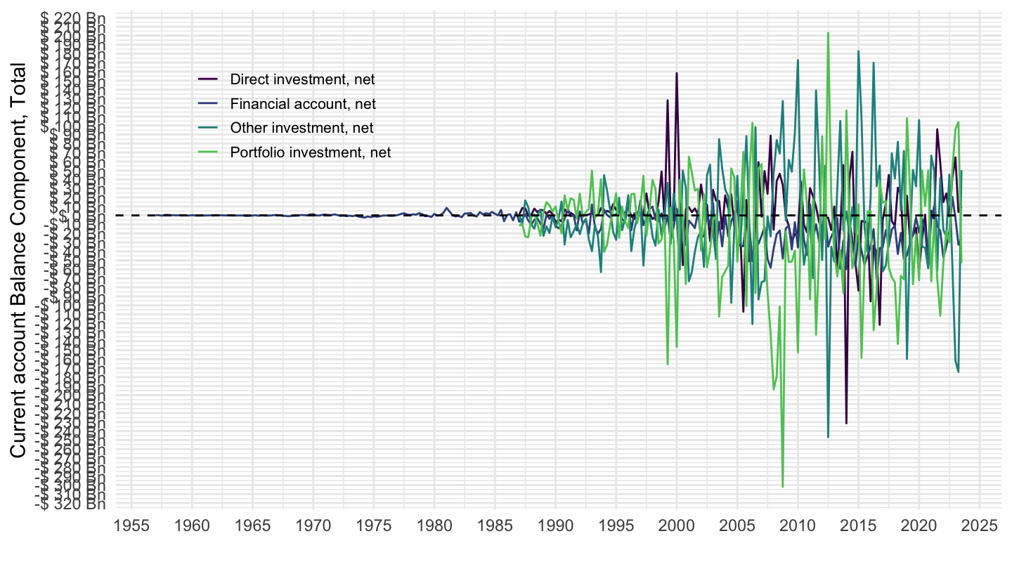

South Korea

MEI_BOP6 %>%
  filter(LOCATION %in% c("KOR"),
         # B6BLTT01: Current account, balance
         # B6BLPI01: Primary income, balance
         # B6BLSI01: Secondary income, balance
         SUBJECT %in% c("B6FADI01", "B6FAPI10", "B6FAOI01", "B6FATT01"),
         # CXCU: US Dollars, sum over component sub-periods, s.a
         MEASURE == "CXCU",
         FREQUENCY == "Q") %>%
  quarter_to_date %>%
  left_join(MEI_BOP6_var$SUBJECT, by = "SUBJECT") %>%
  group_by(LOCATION) %>%
  ggplot(.) + xlab("") + ylab("Current account Balance Component, Total") + 
  geom_line(aes(x = date, y = obsValue/10^3, color = Subject)) + 
  theme_minimal() + scale_color_manual(values = viridis(5)[1:4]) +
  theme(legend.title = element_blank(),
        legend.position = c(0.2, 0.8),
        legend.text = element_text(size = 8),
        legend.key.size = unit(0.9, 'lines')) +
  scale_x_date(breaks = seq(1950, 2100, 5) %>% paste0("-01-01") %>% as.Date,
               labels = date_format("%Y")) +
  scale_y_continuous(breaks = seq(-20000, 400000, 10),
                     labels = dollar_format(accuracy = 1, suffix = " Bn", prefix = "$ ")) +
  geom_hline(yintercept = 0, linetype = "dashed", color = "black")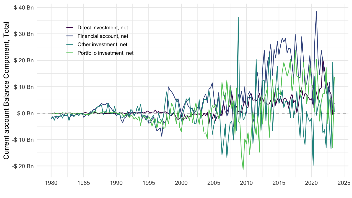

Sweden

MEI_BOP6 %>%
  filter(LOCATION %in% c("SWE"),
         # B6BLTT01: Current account, balance
         # B6BLPI01: Primary income, balance
         # B6BLSI01: Secondary income, balance
         SUBJECT %in% c("B6FADI01", "B6FAPI10", "B6FAOI01", "B6FATT01"),
         # CXCU: US Dollars, sum over component sub-periods, s.a
         MEASURE == "CXCU",
         FREQUENCY == "Q") %>%
  quarter_to_date %>%
  left_join(MEI_BOP6_var$SUBJECT, by = "SUBJECT") %>%
  group_by(LOCATION) %>%
  ggplot(.) + xlab("") + ylab("Current account Balance Component, Total") + 
  geom_line(aes(x = date, y = obsValue/10^3, color = Subject)) + 
  theme_minimal() + scale_color_manual(values = viridis(5)[1:4]) +
  theme(legend.title = element_blank(),
        legend.position = c(0.2, 0.8),
        legend.text = element_text(size = 8),
        legend.key.size = unit(0.9, 'lines')) +
  scale_x_date(breaks = seq(1950, 2100, 5) %>% paste0("-01-01") %>% as.Date,
               labels = date_format("%Y")) +
  scale_y_continuous(breaks = seq(-20000, 400000, 1),
                     labels = dollar_format(accuracy = 1, suffix = " Bn", prefix = "$ ")) +
  geom_hline(yintercept = 0, linetype = "dashed", color = "black")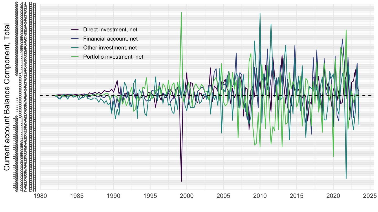

New Zealand

MEI_BOP6 %>%
  filter(LOCATION %in% c("NZL"),
         # B6BLTT01: Current account, balance
         # B6BLPI01: Primary income, balance
         # B6BLSI01: Secondary income, balance
         SUBJECT %in% c("B6FADI01", "B6FAPI10", "B6FAOI01", "B6FATT01"),
         # CXCU: US Dollars, sum over component sub-periods, s.a
         MEASURE == "CXCU",
         FREQUENCY == "Q") %>%
  quarter_to_date %>%
  left_join(MEI_BOP6_var$SUBJECT, by = "SUBJECT") %>%
  group_by(LOCATION) %>%
  ggplot(.) + xlab("") + ylab("Current account Balance Component, Total") + 
  geom_line(aes(x = date, y = obsValue/10^3, color = Subject)) + 
  theme_minimal() + scale_color_manual(values = viridis(5)[1:4]) +
  theme(legend.title = element_blank(),
        legend.position = c(0.2, 0.2),
        legend.text = element_text(size = 8),
        legend.key.size = unit(0.9, 'lines')) +
  scale_x_date(breaks = seq(1950, 2100, 5) %>% paste0("-01-01") %>% as.Date,
               labels = date_format("%Y")) +
  scale_y_continuous(breaks = seq(-20000, 400000, 1),
                     labels = dollar_format(accuracy = 1, suffix = " Bn", prefix = "$ ")) +
  geom_hline(yintercept = 0, linetype = "dashed", color = "black")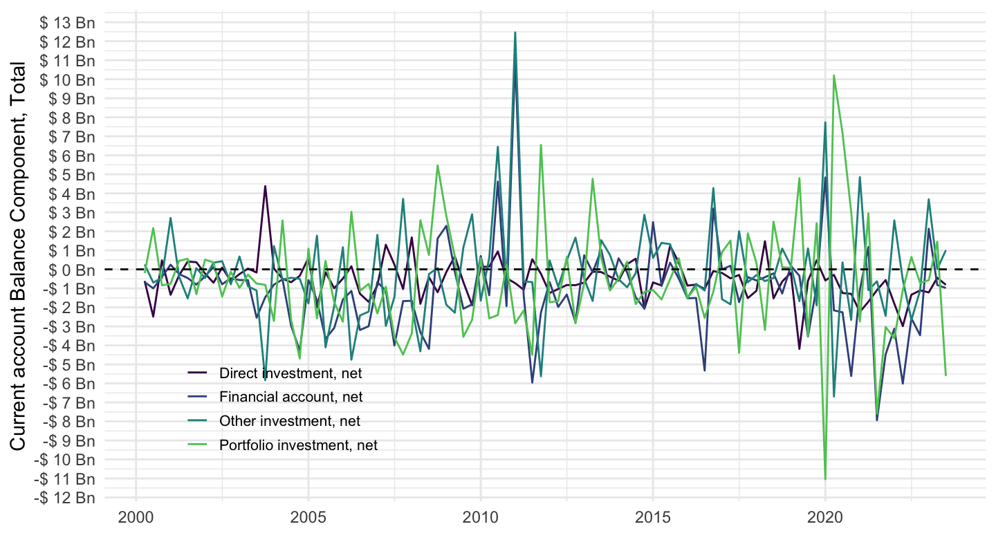

Canada

MEI_BOP6 %>%
  filter(LOCATION %in% c("CAN"),
         # B6BLTT01: Current account, balance
         # B6BLPI01: Primary income, balance
         # B6BLSI01: Secondary income, balance
         SUBJECT %in% c("B6FADI01", "B6FAPI10", "B6FAOI01", "B6FATT01"),
         # CXCU: US Dollars, sum over component sub-periods, s.a
         MEASURE == "CXCU",
         FREQUENCY == "Q") %>%
  quarter_to_date %>%
  left_join(MEI_BOP6_var$SUBJECT, by = "SUBJECT") %>%
  group_by(LOCATION) %>%
  ggplot(.) + xlab("") + ylab("Current account Balance Component, Total") + 
  geom_line(aes(x = date, y = obsValue/10^3, color = Subject)) + 
  theme_minimal() + scale_color_manual(values = viridis(5)[1:4]) +
  theme(legend.title = element_blank(),
        legend.position = c(0.2, 0.8),
        legend.text = element_text(size = 8),
        legend.key.size = unit(0.9, 'lines')) +
  scale_x_date(breaks = seq(1950, 2100, 5) %>% paste0("-01-01") %>% as.Date,
               labels = date_format("%Y")) +
  scale_y_continuous(breaks = seq(-20000, 400000, 5),
                     labels = dollar_format(accuracy = 1, suffix = " Bn", prefix = "$ ")) +
  geom_hline(yintercept = 0, linetype = "dashed", color = "black")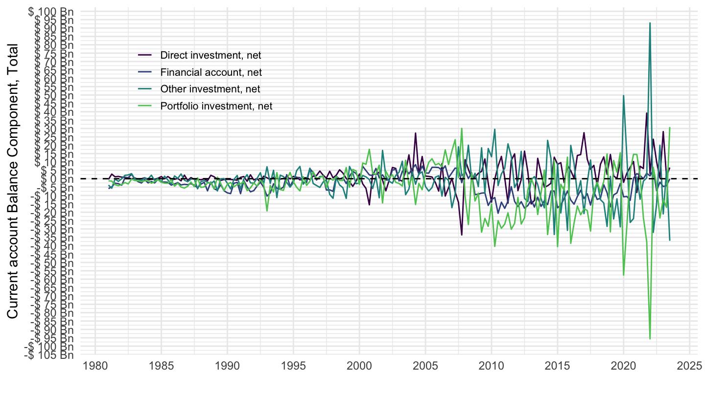

Australia

All

MEI_BOP6 %>%
  filter(LOCATION %in% c("AUS"),
         # B6BLTT01: Current account, balance
         # B6BLPI01: Primary income, balance
         # B6BLSI01: Secondary income, balance
         SUBJECT %in% c("B6FADI01", "B6FAPI10", "B6FAOI01", "B6FATT01"),
         # CXCU: US Dollars, sum over component sub-periods, s.a
         MEASURE == "CXCU",
         FREQUENCY == "Q") %>%
  quarter_to_date %>%
  left_join(MEI_BOP6_var$SUBJECT, by = "SUBJECT") %>%
  group_by(LOCATION) %>%
  ggplot(.) + xlab("") + ylab("Current account Balance Component, Total") + 
  geom_line(aes(x = date, y = obsValue/10^3, color = Subject)) + 
  theme_minimal() + scale_color_manual(values = viridis(5)[1:4]) +
  theme(legend.title = element_blank(),
        legend.position = c(0.2, 0.8),
        legend.text = element_text(size = 8),
        legend.key.size = unit(0.9, 'lines')) +
  scale_x_date(breaks = seq(1950, 2100, 5) %>% paste0("-01-01") %>% as.Date,
               labels = date_format("%Y")) +
  scale_y_continuous(breaks = seq(-20000, 400000, 10),
                     labels = dollar_format(accuracy = 1, suffix = " Bn", prefix = "$ ")) +
  geom_hline(yintercept = 0, linetype = "dashed", color = "black")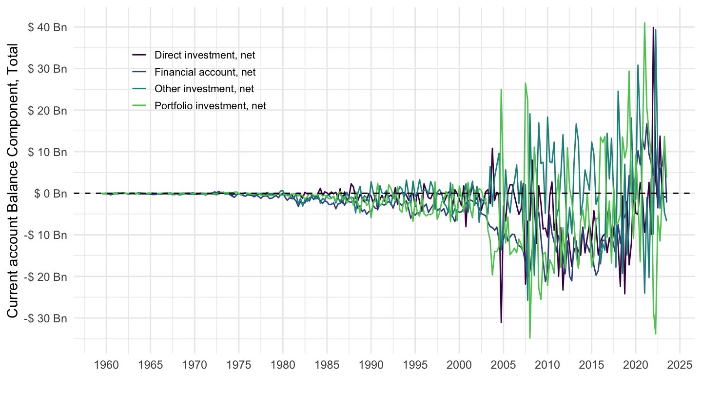

2010

MEI_BOP6 %>%
  filter(LOCATION %in% c("AUS"),
         # B6BLTT01: Current account, balance
         # B6BLPI01: Primary income, balance
         # B6BLSI01: Secondary income, balance
         SUBJECT %in% c("B6FADI01", "B6FAPI10", "B6FAOI01", "B6FATT01"),
         # CXCU: US Dollars, sum over component sub-periods, s.a
         MEASURE == "CXCU",
         FREQUENCY == "Q") %>%
  quarter_to_date %>%
  filter(date >= as.Date("2010-01-01")) %>%
  left_join(MEI_BOP6_var$SUBJECT, by = "SUBJECT") %>%
  group_by(LOCATION) %>%
  ggplot(.) + xlab("") + ylab("Current account Balance Component, Total") + 
  geom_line(aes(x = date, y = obsValue/10^3, color = Subject)) + 
  theme_minimal() + scale_color_manual(values = viridis(5)[1:4]) +
  theme(legend.title = element_blank(),
        legend.position = c(0.2, 0.9),
        legend.text = element_text(size = 8),
        legend.key.size = unit(0.9, 'lines')) +
  scale_x_date(breaks = seq(1950, 2100, 1) %>% paste0("-01-01") %>% as.Date,
               labels = date_format("%Y")) +
  scale_y_continuous(breaks = seq(-20000, 400000, 5),
                     labels = dollar_format(accuracy = 1, suffix = " Bn", prefix = "$ ")) +
  geom_hline(yintercept = 0, linetype = "dashed", color = "black")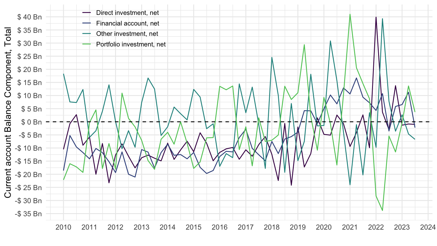

France

MEI_BOP6 %>%
  filter(LOCATION %in% c("FRA"),
         # B6BLTT01: Current account, balance
         # B6BLPI01: Primary income, balance
         # B6BLSI01: Secondary income, balance
         SUBJECT %in% c("B6FADI01", "B6FAPI10", "B6FAOI01", "B6FATT01"),
         # CXCU: US Dollars, sum over component sub-periods, s.a
         MEASURE == "CXCU",
         FREQUENCY == "Q") %>%
  quarter_to_date %>%
  left_join(MEI_BOP6_var$SUBJECT, by = "SUBJECT") %>%
  group_by(LOCATION) %>%
  ggplot(.) + xlab("") + ylab("Current account Balance Component, Total") + 
  geom_line(aes(x = date, y = obsValue/10^3, color = Subject)) + 
  theme_minimal() + scale_color_manual(values = viridis(5)[1:4]) +
  theme(legend.title = element_blank(),
        legend.position = c(0.2, 0.9),
        legend.text = element_text(size = 8),
        legend.key.size = unit(0.9, 'lines')) +
  scale_x_date(breaks = seq(1950, 2100, 2) %>% paste0("-01-01") %>% as.Date,
               labels = date_format("%Y")) +
  scale_y_continuous(breaks = seq(-20000, 400000, 5),
                     labels = dollar_format(accuracy = 1, suffix = " Bn", prefix = "$ ")) +
  geom_hline(yintercept = 0, linetype = "dashed", color = "black")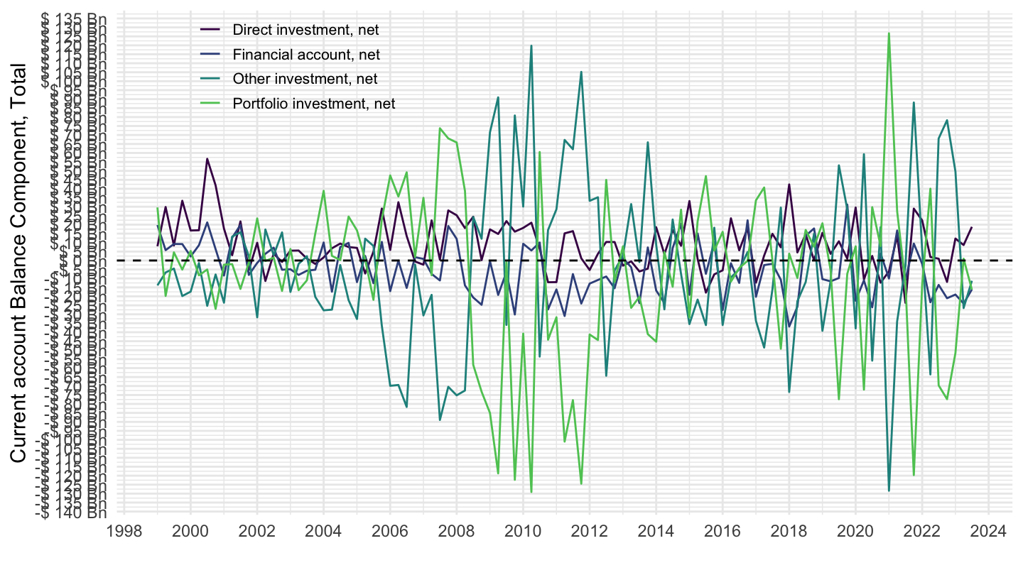

United States

MEI_BOP6 %>%
  filter(LOCATION %in% c("USA"),
         # B6BLTT01: Current account, balance
         # B6BLPI01: Primary income, balance
         # B6BLSI01: Secondary income, balance
         SUBJECT %in% c("B6FADI01", "B6FAPI10", "B6FAOI01", "B6FATT01"),
         # CXCU: US Dollars, sum over component sub-periods, s.a
         MEASURE == "CXCU",
         FREQUENCY == "Q") %>%
  quarter_to_date %>%
  left_join(MEI_BOP6_var$SUBJECT, by = "SUBJECT") %>%
  group_by(LOCATION) %>%
  ggplot(.) + xlab("") + ylab("Current account Balance Component, Total") + 
  geom_line(aes(x = date, y = obsValue/10^3, color = Subject)) + 
  theme_minimal() + scale_color_manual(values = viridis(5)[1:4]) +
  theme(legend.title = element_blank(),
        legend.position = c(0.2, 0.3),
        legend.text = element_text(size = 8),
        legend.key.size = unit(0.9, 'lines')) +
  scale_x_date(breaks = seq(1950, 2100, 5) %>% paste0("-01-01") %>% as.Date,
               labels = date_format("%Y")) +
  scale_y_continuous(breaks = seq(-20000, 400000, 20),
                     labels = dollar_format(accuracy = 1, suffix = " Bn", prefix = "$ ")) +
  geom_hline(yintercept = 0, linetype = "dashed", color = "black")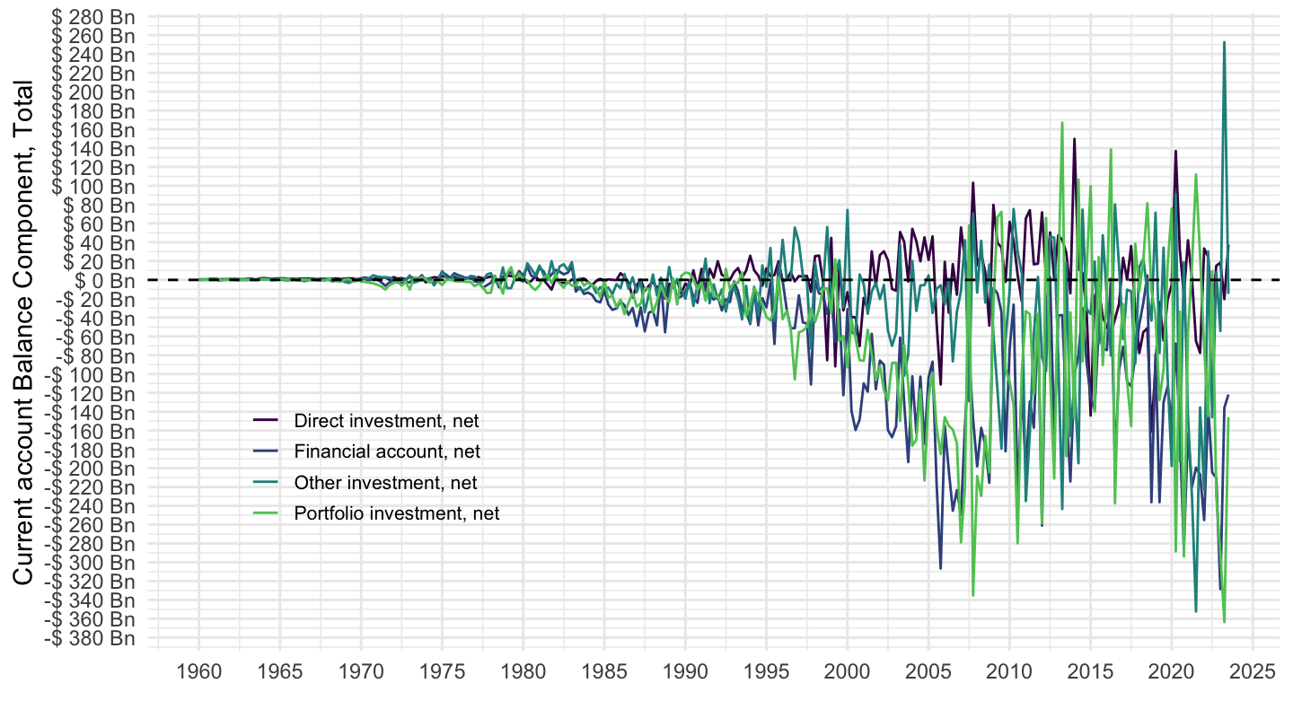

Poland

MEI_BOP6 %>%
  filter(LOCATION %in% c("POL"),
         # B6BLTT01: Current account, balance
         # B6BLPI01: Primary income, balance
         # B6BLSI01: Secondary income, balance
         SUBJECT %in% c("B6FADI01", "B6FAPI10", "B6FAOI01", "B6FATT01"),
         # CXCU: US Dollars, sum over component sub-periods, s.a
         MEASURE == "CXCU",
         FREQUENCY == "Q") %>%
  quarter_to_date %>%
  left_join(MEI_BOP6_var$SUBJECT, by = "SUBJECT") %>%
  group_by(LOCATION) %>%
  ggplot(.) + xlab("") + ylab("Current account Balance Component, Total") + 
  geom_line(aes(x = date, y = obsValue/10^3, color = Subject)) + 
  theme_minimal() + scale_color_manual(values = viridis(5)[1:4]) +
  theme(legend.title = element_blank(),
        legend.position = c(0.2, 0.9),
        legend.text = element_text(size = 8),
        legend.key.size = unit(0.9, 'lines')) +
  scale_x_date(breaks = seq(1950, 2100, 5) %>% paste0("-01-01") %>% as.Date,
               labels = date_format("%Y")) +
  scale_y_continuous(breaks = seq(-20000, 400000, 5),
                     labels = dollar_format(accuracy = 1, suffix = " Bn", prefix = "$ ")) +
  geom_hline(yintercept = 0, linetype = "dashed", color = "black")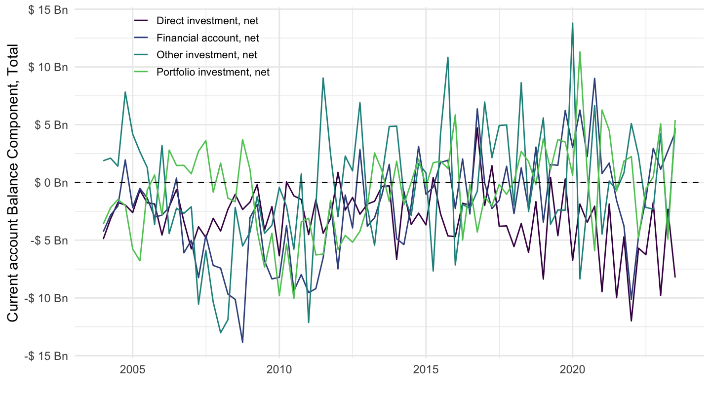

Czech Republic

MEI_BOP6 %>%
  filter(LOCATION %in% c("CZE"),
         # B6BLTT01: Current account, balance
         # B6BLPI01: Primary income, balance
         # B6BLSI01: Secondary income, balance
         SUBJECT %in% c("B6FADI01", "B6FAPI10", "B6FAOI01", "B6FATT01"),
         # CXCU: US Dollars, sum over component sub-periods, s.a
         MEASURE == "CXCU",
         FREQUENCY == "Q") %>%
  quarter_to_date %>%
  left_join(MEI_BOP6_var$SUBJECT, by = "SUBJECT") %>%
  group_by(LOCATION) %>%
  ggplot(.) + xlab("") + ylab("Current account Balance Component, Total") + 
  geom_line(aes(x = date, y = obsValue/10^3, color = Subject)) + 
  theme_minimal() + scale_color_manual(values = viridis(5)[1:4]) +
  theme(legend.title = element_blank(),
        legend.position = c(0.2, 0.3),
        legend.text = element_text(size = 8),
        legend.key.size = unit(0.9, 'lines')) +
  scale_x_date(breaks = seq(1950, 2100, 5) %>% paste0("-01-01") %>% as.Date,
               labels = date_format("%Y")) +
  scale_y_continuous(breaks = seq(-20000, 400000, 1),
                     labels = dollar_format(accuracy = 1, suffix = " Bn", prefix = "$ ")) +
  geom_hline(yintercept = 0, linetype = "dashed", color = "black")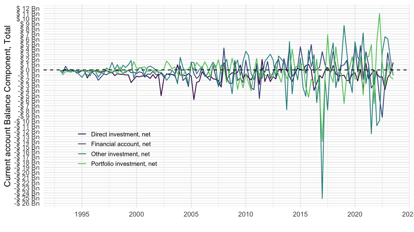

Hungary

MEI_BOP6 %>%
  filter(LOCATION %in% c("HUN"),
         # B6BLTT01: Current account, balance
         # B6BLPI01: Primary income, balance
         # B6BLSI01: Secondary income, balance
         SUBJECT %in% c("B6FADI01", "B6FAPI10", "B6FAOI01", "B6FATT01"),
         # CXCU: US Dollars, sum over component sub-periods, s.a
         MEASURE == "CXCU",
         FREQUENCY == "Q") %>%
  quarter_to_date %>%
  left_join(MEI_BOP6_var$SUBJECT, by = "SUBJECT") %>%
  group_by(LOCATION) %>%
  ggplot(.) + xlab("") + ylab("Current account Balance Component, Total") + 
  geom_line(aes(x = date, y = obsValue/10^3, color = Subject)) + 
  theme_minimal() + scale_color_manual(values = viridis(5)[1:4]) +
  theme(legend.title = element_blank(),
        legend.position = c(0.2, 0.9),
        legend.text = element_text(size = 8),
        legend.key.size = unit(0.9, 'lines')) +
  scale_x_date(breaks = seq(1950, 2100, 5) %>% paste0("-01-01") %>% as.Date,
               labels = date_format("%Y")) +
  scale_y_continuous(breaks = seq(-20000, 400000, 1),
                     labels = dollar_format(accuracy = 1, suffix = " Bn", prefix = "$ ")) +
  geom_hline(yintercept = 0, linetype = "dashed", color = "black")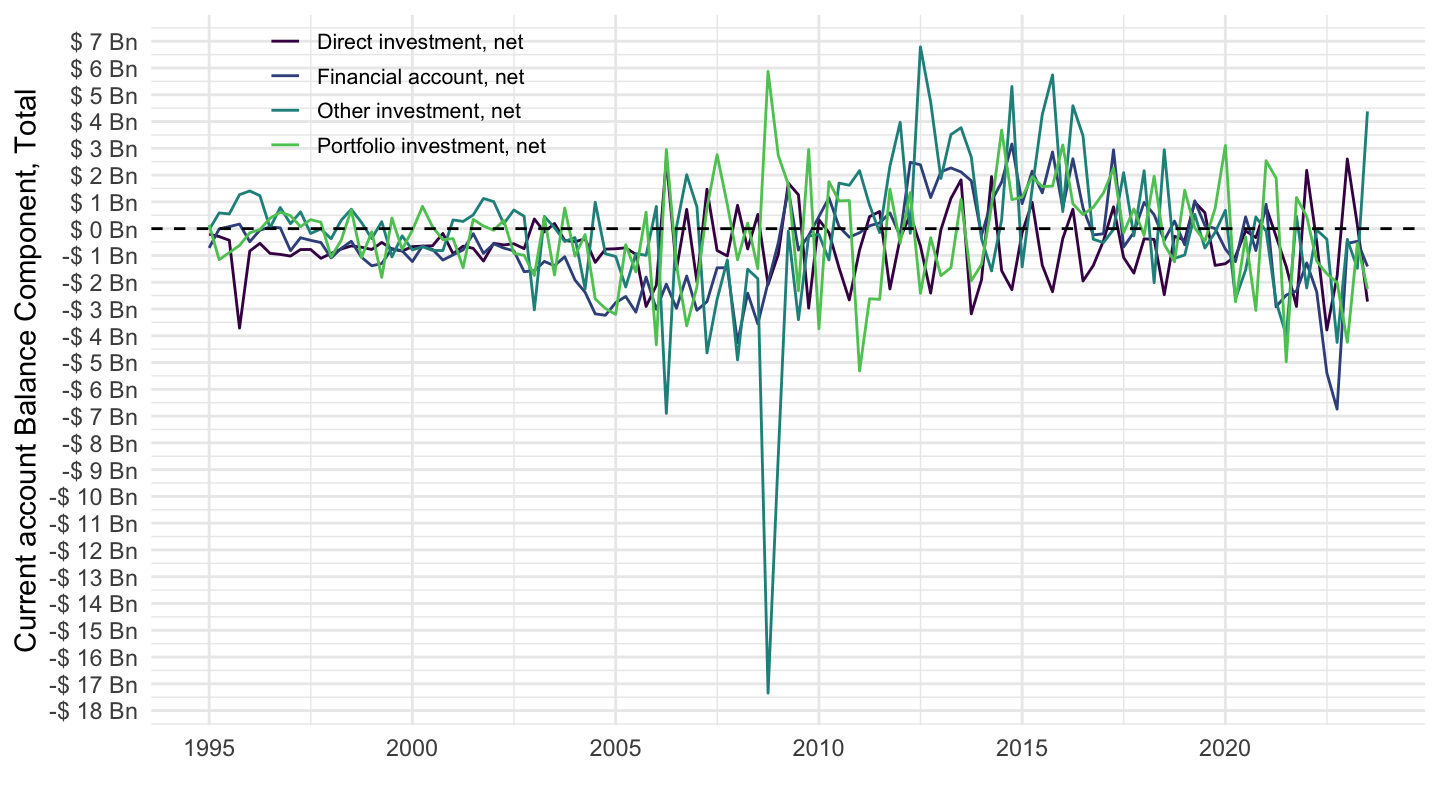

Portugal

MEI_BOP6 %>%
  filter(LOCATION %in% c("PRT"),
         # B6BLTT01: Current account, balance
         # B6BLPI01: Primary income, balance
         # B6BLSI01: Secondary income, balance
         SUBJECT %in% c("B6FADI01", "B6FAPI10", "B6FAOI01", "B6FATT01"),
         # CXCU: US Dollars, sum over component sub-periods, s.a
         MEASURE == "CXCU",
         FREQUENCY == "Q") %>%
  quarter_to_date %>%
  left_join(MEI_BOP6_var$SUBJECT, by = "SUBJECT") %>%
  group_by(LOCATION) %>%
  ggplot(.) + xlab("") + ylab("Current account Balance Component, Total") + 
  geom_line(aes(x = date, y = obsValue/10^3, color = Subject)) + 
  theme_minimal() + scale_color_manual(values = viridis(5)[1:4]) +
  theme(legend.title = element_blank(),
        legend.position = c(0.2, 0.9),
        legend.text = element_text(size = 8),
        legend.key.size = unit(0.9, 'lines')) +
  scale_x_date(breaks = seq(1950, 2100, 2) %>% paste0("-01-01") %>% as.Date,
               labels = date_format("%Y")) +
  scale_y_continuous(breaks = seq(-20000, 400000, 1),
                     labels = dollar_format(accuracy = 1, suffix = " Bn", prefix = "$ ")) +
  geom_hline(yintercept = 0, linetype = "dashed", color = "black")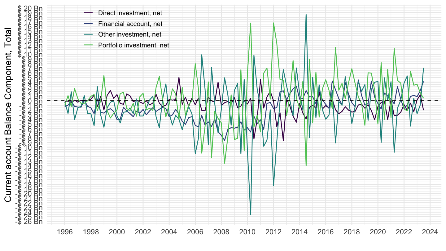

Austria

MEI_BOP6 %>%
  filter(LOCATION %in% c("AUT"),
         # B6BLTT01: Current account, balance
         # B6BLPI01: Primary income, balance
         # B6BLSI01: Secondary income, balance
         SUBJECT %in% c("B6FADI01", "B6FAPI10", "B6FAOI01", "B6FATT01"),
         # CXCU: US Dollars, sum over component sub-periods, s.a
         MEASURE == "CXCU",
         FREQUENCY == "Q") %>%
  quarter_to_date %>%
  left_join(MEI_BOP6_var$SUBJECT, by = "SUBJECT") %>%
  group_by(LOCATION) %>%
  ggplot(.) + xlab("") + ylab("Current account Balance Component, Total") + 
  geom_line(aes(x = date, y = obsValue/10^3, color = Subject)) + 
  theme_minimal() + scale_color_manual(values = viridis(5)[1:4]) +
  theme(legend.title = element_blank(),
        legend.position = c(0.2, 0.8),
        legend.text = element_text(size = 8),
        legend.key.size = unit(0.9, 'lines')) +
  scale_x_date(breaks = seq(1950, 2100, 2) %>% paste0("-01-01") %>% as.Date,
               labels = date_format("%Y")) +
  scale_y_continuous(breaks = seq(-20000, 400000, 1),
                     labels = dollar_format(accuracy = 1, suffix = " Bn", prefix = "$ ")) +
  geom_hline(yintercept = 0, linetype = "dashed", color = "black")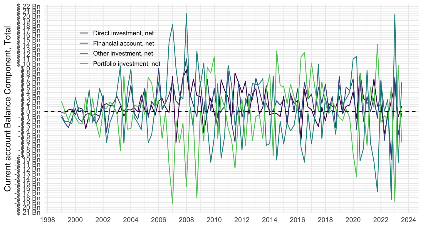

Capital Account Decompositions - Annual

Germany

MEI_BOP6 %>%
  filter(LOCATION %in% c("DEU"),
         # B6FADI01: Current account, balance
         # B6BLPI01: Primary income, balance
         # B6BLSI01: Secondary income, balance
         SUBJECT %in% c("B6FADI01", "B6FAPI10", "B6FAOI01", "B6FATT01"),
         MEASURE == "CXCU",
         # CXCUSA: US Dollars, sum over component sub-periods, s.a
         FREQUENCY == "A") %>%
  year_to_date %>%
  left_join(MEI_BOP6_var$SUBJECT, by = "SUBJECT") %>%
  ggplot(.) + xlab("") + ylab("Current account Balance Component, Total") + 
  geom_line(aes(x = date, y = obsValue/10^3, color = Subject)) + 
  theme_minimal() + scale_color_manual(values = viridis(5)[1:4]) +
  theme(legend.title = element_blank(),
        legend.position = c(0.2, 0.8),
        legend.text = element_text(size = 8),
        legend.key.size = unit(0.9, 'lines')) +
  scale_x_date(breaks = seq(1950, 2100, 5) %>% paste0("-01-01") %>% as.Date,
               labels = date_format("%Y")) +
  scale_y_continuous(breaks = seq(-20000, 400000, 50),
                     labels = dollar_format(accuracy = 1, suffix = " Bn", prefix = "$ ")) +
  geom_hline(yintercept = 0, linetype = "dashed", color = "black")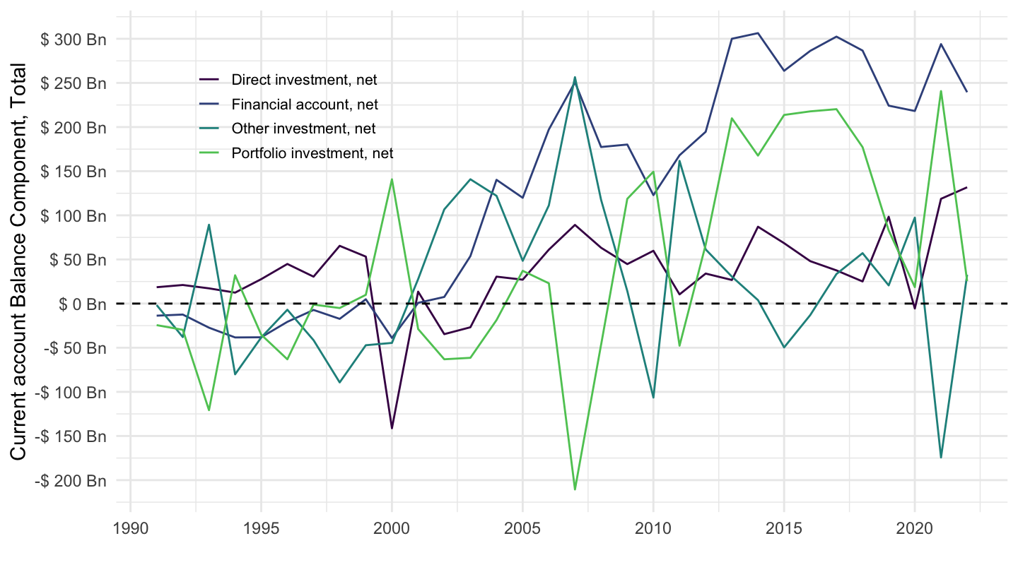

Euro Area

MEI_BOP6 %>%
  filter(LOCATION %in% c("EA20"),
         # B6BLTT01: Current account, balance
         # B6BLPI01: Primary income, balance
         # B6BLSI01: Secondary income, balance
         SUBJECT %in% c("B6FADI01", "B6FAPI10", "B6FAOI01", "B6FATT01"),
         # CXCU: US Dollars, sum over component sub-periods, s.a
         MEASURE == "CXCU",
         FREQUENCY == "A") %>%
  year_to_date %>%
  left_join(MEI_BOP6_var$SUBJECT, by = "SUBJECT") %>%
  group_by(LOCATION) %>%
  ggplot(.) + xlab("") + ylab("Current account Balance Component, Total") + 
  geom_line(aes(x = date, y = obsValue/10^3, color = Subject)) + 
  theme_minimal() + scale_color_manual(values = viridis(5)[1:4]) +
  theme(legend.title = element_blank(),
        legend.position = c(0.2, 0.8),
        legend.text = element_text(size = 8),
        legend.key.size = unit(0.9, 'lines')) +
  scale_x_date(breaks = seq(1950, 2100, 2) %>% paste0("-01-01") %>% as.Date,
               labels = date_format("%Y")) +
  scale_y_continuous(breaks = seq(-20000, 400000, 50),
                     labels = dollar_format(accuracy = 1, suffix = " Bn", prefix = "$ ")) +
  geom_hline(yintercept = 0, linetype = "dashed", color = "black")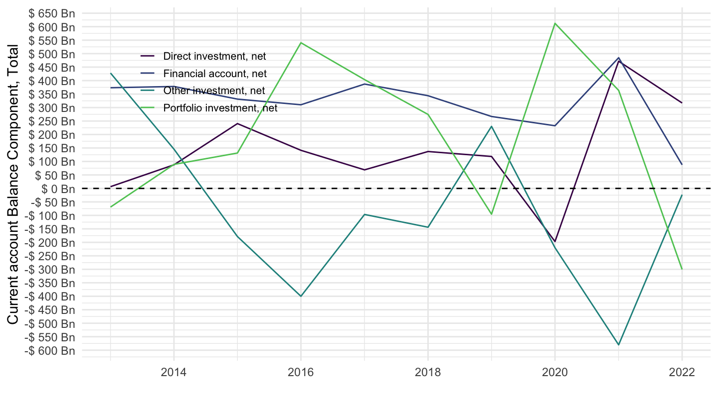

China

MEI_BOP6 %>%
  filter(LOCATION %in% c("CHN"),
         # B6BLTT01: Current account, balance
         # B6BLPI01: Primary income, balance
         # B6BLSI01: Secondary income, balance
         SUBJECT %in% c("B6FADI01", "B6FAPI10", "B6FAOI01", "B6FATT01"),
         # CXCU: US Dollars, sum over component sub-periods, s.a
         MEASURE == "CXCU",
         FREQUENCY == "A") %>%
  year_to_date %>%
  left_join(MEI_BOP6_var$SUBJECT, by = "SUBJECT") %>%
  group_by(LOCATION) %>%
  ggplot(.) + xlab("") + ylab("Current account Balance Component, Total") + 
  geom_line(aes(x = date, y = obsValue/10^3, color = Subject)) + 
  theme_minimal() + scale_color_manual(values = viridis(5)[1:4]) +
  theme(legend.title = element_blank(),
        legend.position = c(0.2, 0.8),
        legend.text = element_text(size = 8),
        legend.key.size = unit(0.9, 'lines')) +
  scale_x_date(breaks = seq(1950, 2100, 5) %>% paste0("-01-01") %>% as.Date,
               labels = date_format("%Y")) +
  scale_y_continuous(breaks = seq(-20000, 400000, 50),
                     labels = dollar_format(accuracy = 1, suffix = " Bn", prefix = "$ ")) +
  geom_hline(yintercept = 0, linetype = "dashed", color = "black")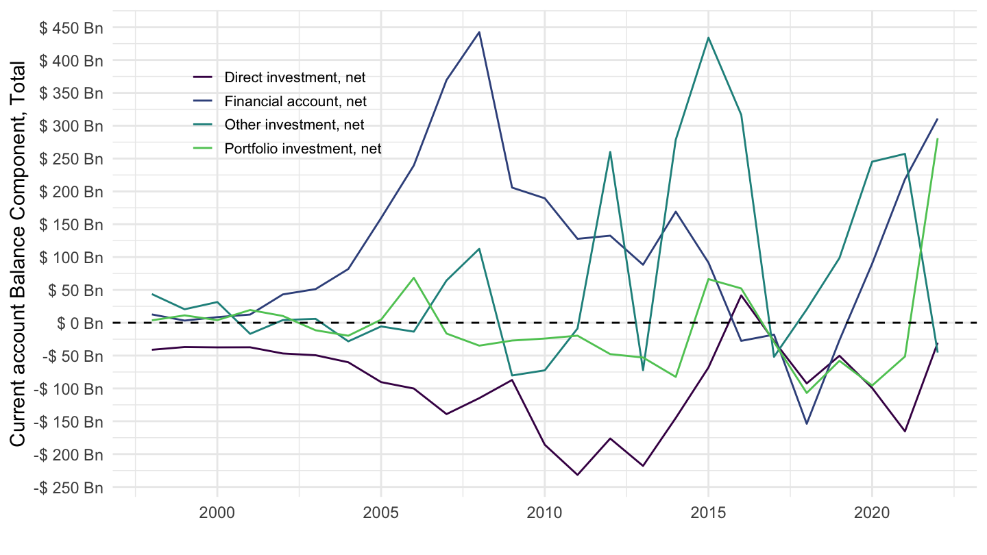

United Kingdom

MEI_BOP6 %>%
  filter(LOCATION %in% c("GBR"),
         # B6BLTT01: Current account, balance
         # B6BLPI01: Primary income, balance
         # B6BLSI01: Secondary income, balance
         SUBJECT %in% c("B6FADI01", "B6FAPI10", "B6FAOI01", "B6FATT01"),
         # CXCU: US Dollars, sum over component sub-periods, s.a
         MEASURE == "CXCU",
         FREQUENCY == "A") %>%
  year_to_date %>%
  left_join(MEI_BOP6_var$SUBJECT, by = "SUBJECT") %>%
  group_by(LOCATION) %>%
  ggplot(.) + xlab("") + ylab("Current account Balance Component, Total") + 
  geom_line(aes(x = date, y = obsValue/10^3, color = Subject)) + 
  theme_minimal() + scale_color_manual(values = viridis(5)[1:4]) +
  theme(legend.title = element_blank(),
        legend.position = c(0.2, 0.8),
        legend.text = element_text(size = 8),
        legend.key.size = unit(0.9, 'lines')) +
  scale_x_date(breaks = seq(1950, 2100, 5) %>% paste0("-01-01") %>% as.Date,
               labels = date_format("%Y")) +
  scale_y_continuous(breaks = seq(-20000, 400000, 50),
                     labels = dollar_format(accuracy = 1, suffix = " Bn", prefix = "$ ")) +
  geom_hline(yintercept = 0, linetype = "dashed", color = "black")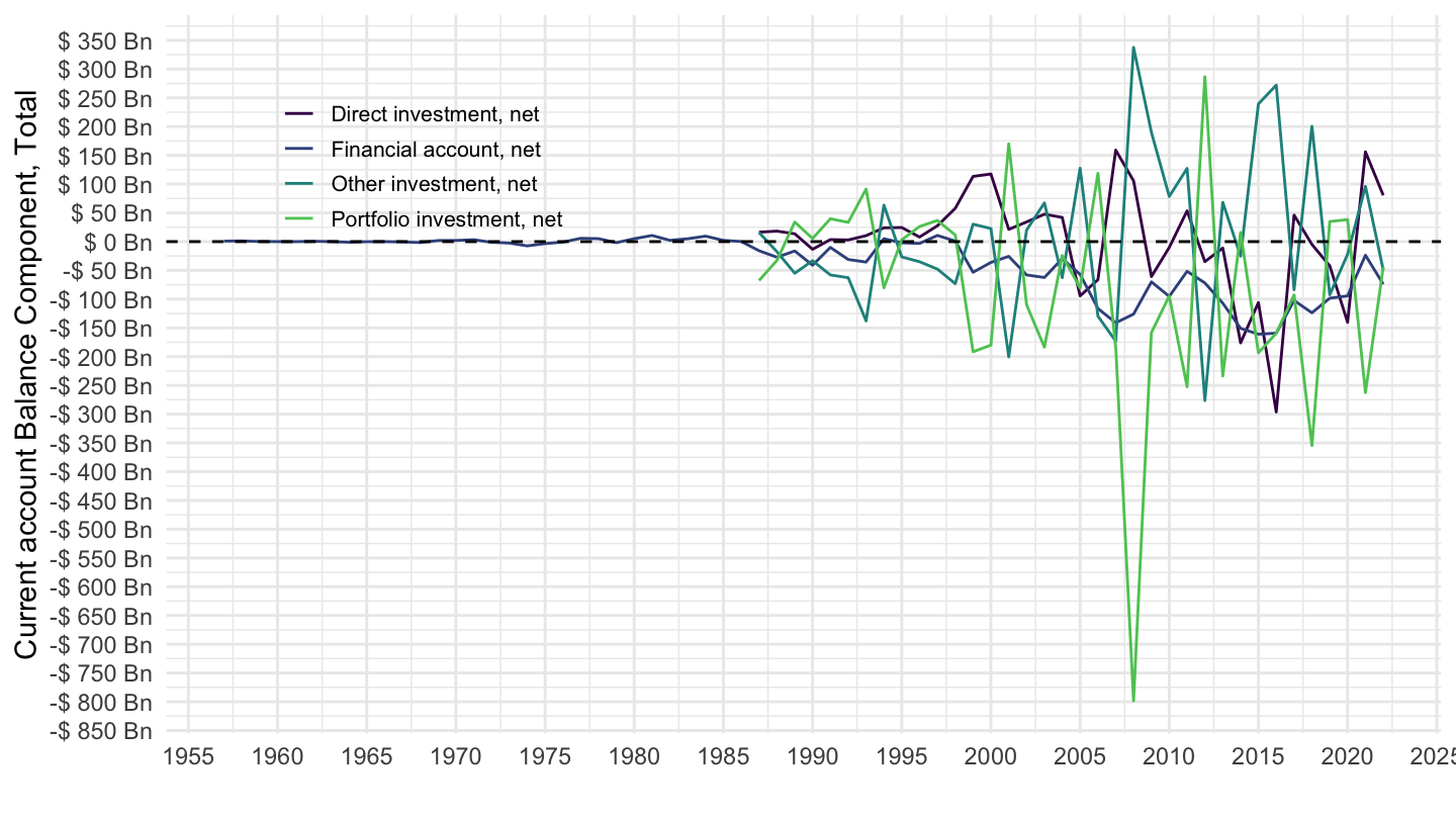

South Korea

MEI_BOP6 %>%
  filter(LOCATION %in% c("KOR"),
         # B6BLTT01: Current account, balance
         # B6BLPI01: Primary income, balance
         # B6BLSI01: Secondary income, balance
         SUBJECT %in% c("B6FADI01", "B6FAPI10", "B6FAOI01", "B6FATT01"),
         # CXCU: US Dollars, sum over component sub-periods, s.a
         MEASURE == "CXCU",
         FREQUENCY == "A") %>%
  year_to_date %>%
  left_join(MEI_BOP6_var$SUBJECT, by = "SUBJECT") %>%
  group_by(LOCATION) %>%
  ggplot(.) + xlab("") + ylab("Current account Balance Component, Total") + 
  geom_line(aes(x = date, y = obsValue/10^3, color = Subject)) + 
  theme_minimal() + scale_color_manual(values = viridis(5)[1:4]) +
  theme(legend.title = element_blank(),
        legend.position = c(0.2, 0.8),
        legend.text = element_text(size = 8),
        legend.key.size = unit(0.9, 'lines')) +
  scale_x_date(breaks = seq(1950, 2100, 5) %>% paste0("-01-01") %>% as.Date,
               labels = date_format("%Y")) +
  scale_y_continuous(breaks = seq(-20000, 400000, 10),
                     labels = dollar_format(accuracy = 1, suffix = " Bn", prefix = "$ ")) +
  geom_hline(yintercept = 0, linetype = "dashed", color = "black")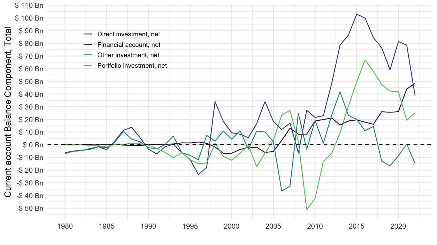

Sweden

MEI_BOP6 %>%
  filter(LOCATION %in% c("SWE"),
         # B6BLTT01: Current account, balance
         # B6BLPI01: Primary income, balance
         # B6BLSI01: Secondary income, balance
         SUBJECT %in% c("B6FADI01", "B6FAPI10", "B6FAOI01", "B6FATT01"),
         # CXCU: US Dollars, sum over component sub-periods, s.a
         MEASURE == "CXCU",
         FREQUENCY == "A") %>%
  year_to_date %>%
  left_join(MEI_BOP6_var$SUBJECT, by = "SUBJECT") %>%
  group_by(LOCATION) %>%
  ggplot(.) + xlab("") + ylab("Current account Balance Component, Total") + 
  geom_line(aes(x = date, y = obsValue/10^3, color = Subject)) + 
  theme_minimal() + scale_color_manual(values = viridis(5)[1:4]) +
  theme(legend.title = element_blank(),
        legend.position = c(0.2, 0.8),
        legend.text = element_text(size = 8),
        legend.key.size = unit(0.9, 'lines')) +
  scale_x_date(breaks = seq(1950, 2100, 5) %>% paste0("-01-01") %>% as.Date,
               labels = date_format("%Y")) +
  scale_y_continuous(breaks = seq(-20000, 400000, 20),
                     labels = dollar_format(accuracy = 1, suffix = " Bn", prefix = "$ ")) +
  geom_hline(yintercept = 0, linetype = "dashed", color = "black")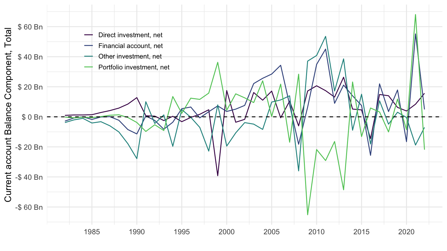

New Zealand

MEI_BOP6 %>%
  filter(LOCATION %in% c("NZL"),
         # B6BLTT01: Current account, balance
         # B6BLPI01: Primary income, balance
         # B6BLSI01: Secondary income, balance
         SUBJECT %in% c("B6FADI01", "B6FAPI10", "B6FAOI01", "B6FATT01"),
         # CXCU: US Dollars, sum over component sub-periods, s.a
         MEASURE == "CXCU",
         FREQUENCY == "A") %>%
  year_to_date %>%
  left_join(MEI_BOP6_var$SUBJECT, by = "SUBJECT") %>%
  group_by(LOCATION) %>%
  ggplot(.) + xlab("") + ylab("Current account Balance Component, Total") + 
  geom_line(aes(x = date, y = obsValue/10^3, color = Subject)) + 
  theme_minimal() + scale_color_manual(values = viridis(5)[1:4]) +
  theme(legend.title = element_blank(),
        legend.position = c(0.2, 0.2),
        legend.text = element_text(size = 8),
        legend.key.size = unit(0.9, 'lines')) +
  scale_x_date(breaks = seq(1950, 2100, 5) %>% paste0("-01-01") %>% as.Date,
               labels = date_format("%Y")) +
  scale_y_continuous(breaks = seq(-20000, 400000, 1),
                     labels = dollar_format(accuracy = 1, suffix = " Bn", prefix = "$ ")) +
  geom_hline(yintercept = 0, linetype = "dashed", color = "black")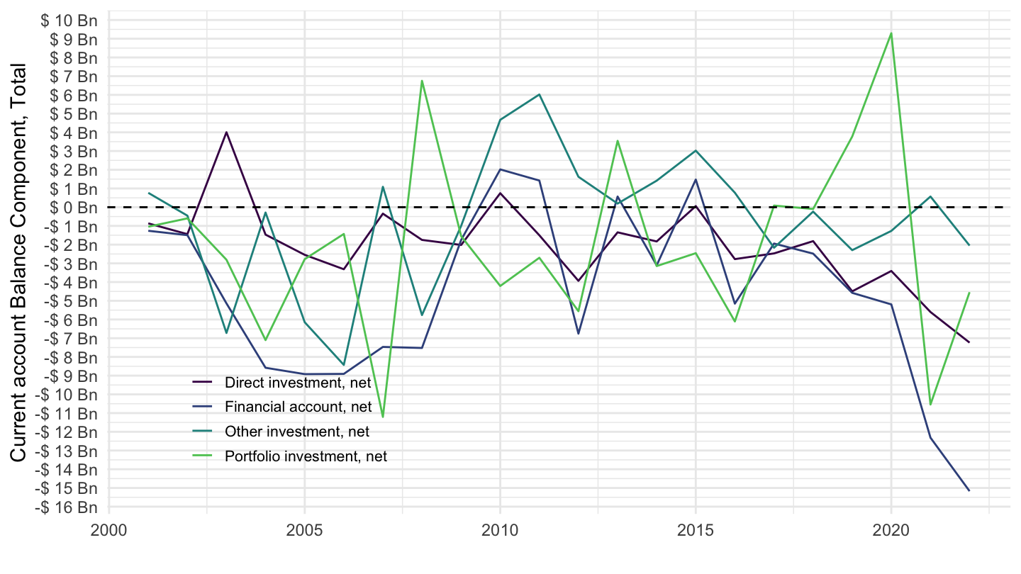

Canada

MEI_BOP6 %>%
  filter(LOCATION %in% c("CAN"),
         # B6BLTT01: Current account, balance
         # B6BLPI01: Primary income, balance
         # B6BLSI01: Secondary income, balance
         SUBJECT %in% c("B6FADI01", "B6FAPI10", "B6FAOI01", "B6FATT01"),
         # CXCU: US Dollars, sum over component sub-periods, s.a
         MEASURE == "CXCU",
         FREQUENCY == "A") %>%
  year_to_date %>%
  left_join(MEI_BOP6_var$SUBJECT, by = "SUBJECT") %>%
  group_by(LOCATION) %>%
  ggplot(.) + xlab("") + ylab("Current account Balance Component, Total") + 
  geom_line(aes(x = date, y = obsValue/10^3, color = Subject)) + 
  theme_minimal() + scale_color_manual(values = viridis(5)[1:4]) +
  theme(legend.title = element_blank(),
        legend.position = c(0.2, 0.8),
        legend.text = element_text(size = 8),
        legend.key.size = unit(0.9, 'lines')) +
  scale_x_date(breaks = seq(1950, 2100, 5) %>% paste0("-01-01") %>% as.Date,
               labels = date_format("%Y")) +
  scale_y_continuous(breaks = seq(-20000, 400000, 20),
                     labels = dollar_format(accuracy = 1, suffix = " Bn", prefix = "$ ")) +
  geom_hline(yintercept = 0, linetype = "dashed", color = "black")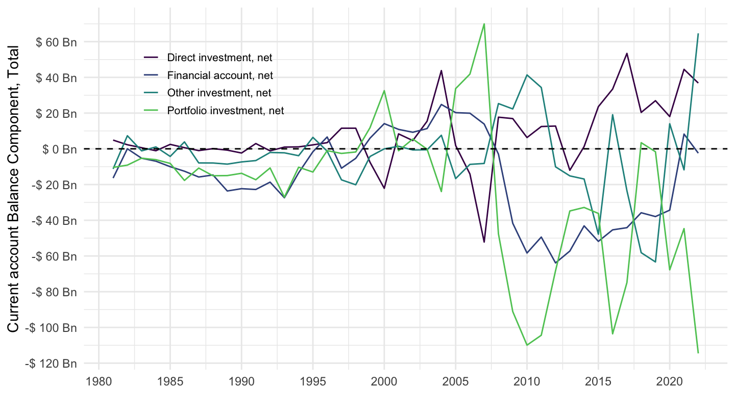

Australia

All

MEI_BOP6 %>%
  filter(LOCATION %in% c("AUS"),
         # B6BLTT01: Current account, balance
         # B6BLPI01: Primary income, balance
         # B6BLSI01: Secondary income, balance
         SUBJECT %in% c("B6FADI01", "B6FAPI10", "B6FAOI01", "B6FATT01"),
         # CXCU: US Dollars, sum over component sub-periods, s.a
         MEASURE == "CXCU",
         FREQUENCY == "A") %>%
  year_to_date %>%
  left_join(MEI_BOP6_var$SUBJECT, by = "SUBJECT") %>%
  group_by(LOCATION) %>%
  ggplot(.) + xlab("") + ylab("Current account Balance Component, Total") + 
  geom_line(aes(x = date, y = obsValue/10^3, color = Subject)) + 
  theme_minimal() + scale_color_manual(values = viridis(5)[1:4]) +
  theme(legend.title = element_blank(),
        legend.position = c(0.2, 0.8),
        legend.text = element_text(size = 8),
        legend.key.size = unit(0.9, 'lines')) +
  scale_x_date(breaks = seq(1950, 2100, 5) %>% paste0("-01-01") %>% as.Date,
               labels = date_format("%Y")) +
  scale_y_continuous(breaks = seq(-20000, 400000, 10),
                     labels = dollar_format(accuracy = 1, suffix = " Bn", prefix = "$ ")) +
  geom_hline(yintercept = 0, linetype = "dashed", color = "black")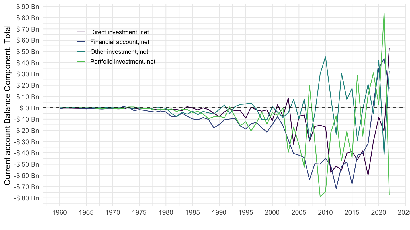

2010

MEI_BOP6 %>%
  filter(LOCATION %in% c("AUS"),
         # B6BLTT01: Current account, balance
         # B6BLPI01: Primary income, balance
         # B6BLSI01: Secondary income, balance
         SUBJECT %in% c("B6FADI01", "B6FAPI10", "B6FAOI01", "B6FATT01"),
         # CXCU: US Dollars, sum over component sub-periods, s.a
         MEASURE == "CXCU",
         FREQUENCY == "A") %>%
  year_to_date %>%
  filter(date >= as.Date("2010-01-01")) %>%
  left_join(MEI_BOP6_var$SUBJECT, by = "SUBJECT") %>%
  group_by(LOCATION) %>%
  ggplot(.) + xlab("") + ylab("Current account Balance Component, Total") + 
  geom_line(aes(x = date, y = obsValue/10^3, color = Subject)) + 
  theme_minimal() + scale_color_manual(values = viridis(5)[1:4]) +
  theme(legend.title = element_blank(),
        legend.position = c(0.2, 0.9),
        legend.text = element_text(size = 8),
        legend.key.size = unit(0.9, 'lines')) +
  scale_x_date(breaks = seq(1950, 2100, 1) %>% paste0("-01-01") %>% as.Date,
               labels = date_format("%Y")) +
  scale_y_continuous(breaks = seq(-20000, 400000, 5),
                     labels = dollar_format(accuracy = 1, suffix = " Bn", prefix = "$ ")) +
  geom_hline(yintercept = 0, linetype = "dashed", color = "black")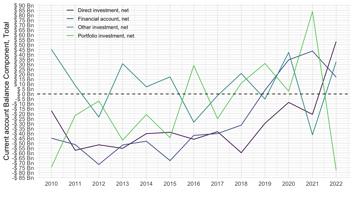

France

MEI_BOP6 %>%
  filter(LOCATION %in% c("FRA"),
         # B6BLTT01: Current account, balance
         # B6BLPI01: Primary income, balance
         # B6BLSI01: Secondary income, balance
         SUBJECT %in% c("B6FADI01", "B6FAPI10", "B6FAOI01", "B6FATT01"),
         # CXCU: US Dollars, sum over component sub-periods, s.a
         MEASURE == "CXCU",
         FREQUENCY == "A") %>%
  year_to_date %>%
  left_join(MEI_BOP6_var$SUBJECT, by = "SUBJECT") %>%
  group_by(LOCATION) %>%
  ggplot(.) + xlab("") + ylab("Current account Balance Component, Total") + 
  geom_line(aes(x = date, y = obsValue/10^3, color = Subject)) + 
  theme_minimal() + scale_color_manual(values = viridis(5)[1:4]) +
  theme(legend.title = element_blank(),
        legend.position = c(0.2, 0.9),
        legend.text = element_text(size = 8),
        legend.key.size = unit(0.9, 'lines')) +
  scale_x_date(breaks = seq(1950, 2100, 2) %>% paste0("-01-01") %>% as.Date,
               labels = date_format("%Y")) +
  scale_y_continuous(breaks = seq(-20000, 400000, 50),
                     labels = dollar_format(accuracy = 1, suffix = " Bn", prefix = "$ ")) +
  geom_hline(yintercept = 0, linetype = "dashed", color = "black")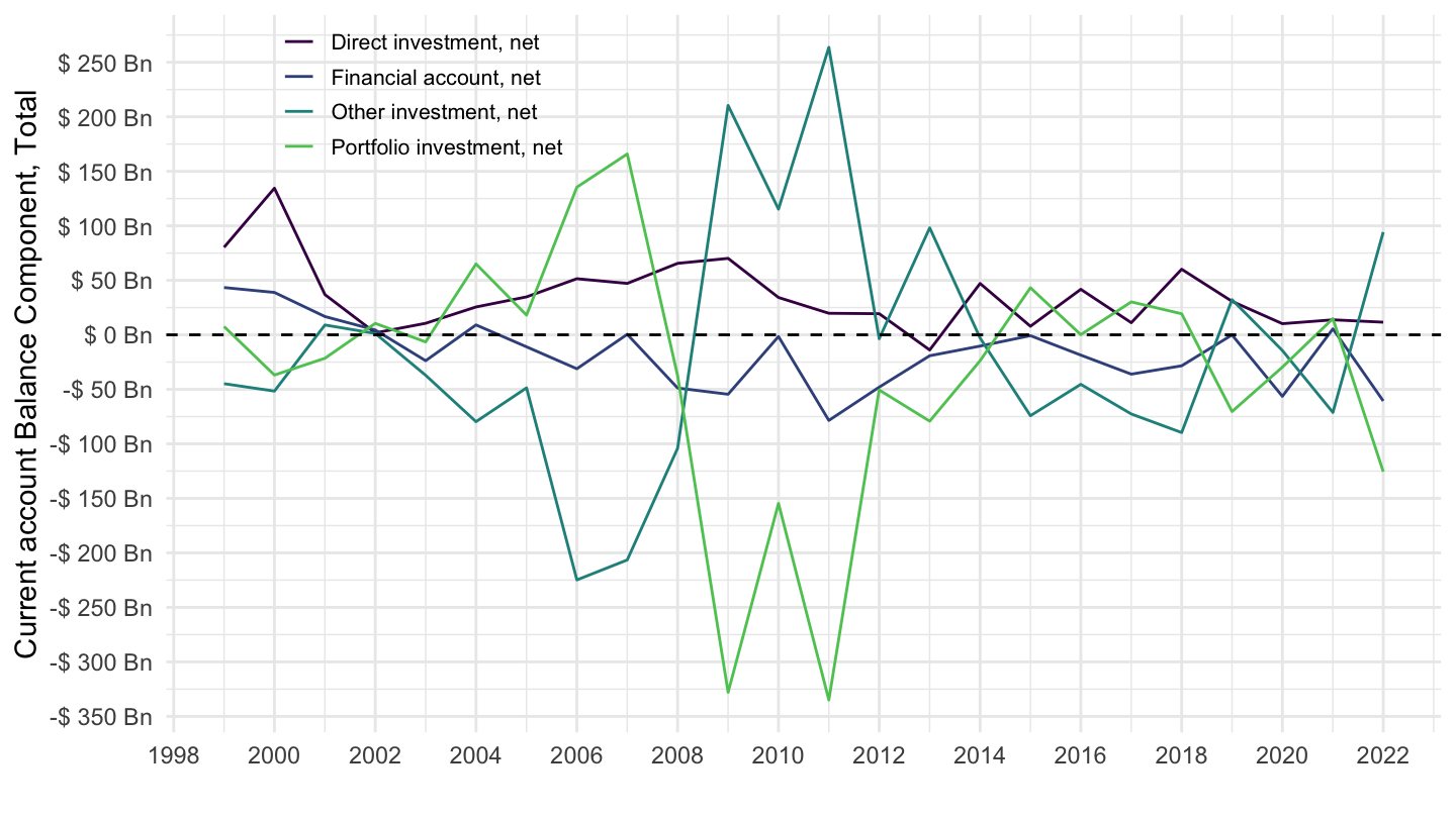

United States

MEI_BOP6 %>%
  filter(LOCATION %in% c("USA"),
         # B6BLTT01: Current account, balance
         # B6BLPI01: Primary income, balance
         # B6BLSI01: Secondary income, balance
         SUBJECT %in% c("B6FADI01", "B6FAPI10", "B6FAOI01", "B6FATT01"),
         # CXCU: US Dollars, sum over component sub-periods, s.a
         MEASURE == "CXCU",
         FREQUENCY == "A") %>%
  year_to_date %>%
  left_join(MEI_BOP6_var$SUBJECT, by = "SUBJECT") %>%
  group_by(LOCATION) %>%
  ggplot(.) + xlab("") + ylab("Current account Balance Component, Total") + 
  geom_line(aes(x = date, y = obsValue/10^3, color = Subject)) + 
  theme_minimal() + scale_color_manual(values = viridis(5)[1:4]) +
  theme(legend.title = element_blank(),
        legend.position = c(0.2, 0.3),
        legend.text = element_text(size = 8),
        legend.key.size = unit(0.9, 'lines')) +
  scale_x_date(breaks = seq(1950, 2100, 5) %>% paste0("-01-01") %>% as.Date,
               labels = date_format("%Y")) +
  scale_y_continuous(breaks = seq(-20000, 400000, 50),
                     labels = dollar_format(accuracy = 1, suffix = " Bn", prefix = "$ ")) +
  geom_hline(yintercept = 0, linetype = "dashed", color = "black")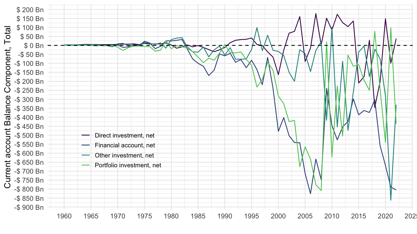

Poland

MEI_BOP6 %>%
  filter(LOCATION %in% c("POL"),
         # B6BLTT01: Current account, balance
         # B6BLPI01: Primary income, balance
         # B6BLSI01: Secondary income, balance
         SUBJECT %in% c("B6FADI01", "B6FAPI10", "B6FAOI01", "B6FATT01"),
         # CXCU: US Dollars, sum over component sub-periods, s.a
         MEASURE == "CXCU",
         FREQUENCY == "A") %>%
  year_to_date %>%
  left_join(MEI_BOP6_var$SUBJECT, by = "SUBJECT") %>%
  group_by(LOCATION) %>%
  ggplot(.) + xlab("") + ylab("Current account Balance Component, Total") + 
  geom_line(aes(x = date, y = obsValue/10^3, color = Subject)) + 
  theme_minimal() + scale_color_manual(values = viridis(5)[1:4]) +
  theme(legend.title = element_blank(),
        legend.position = c(0.2, 0.9),
        legend.text = element_text(size = 8),
        legend.key.size = unit(0.9, 'lines')) +
  scale_x_date(breaks = seq(1950, 2100, 5) %>% paste0("-01-01") %>% as.Date,
               labels = date_format("%Y")) +
  scale_y_continuous(breaks = seq(-20000, 400000, 5),
                     labels = dollar_format(accuracy = 1, suffix = " Bn", prefix = "$ ")) +
  geom_hline(yintercept = 0, linetype = "dashed", color = "black")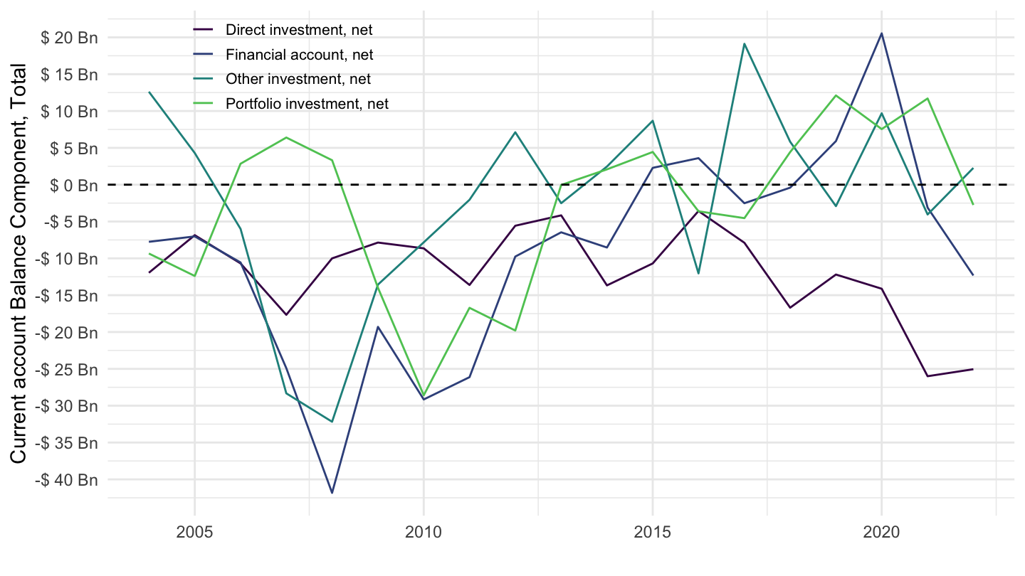

Czech Republic

MEI_BOP6 %>%
  filter(LOCATION %in% c("CZE"),
         # B6BLTT01: Current account, balance
         # B6BLPI01: Primary income, balance
         # B6BLSI01: Secondary income, balance
         SUBJECT %in% c("B6FADI01", "B6FAPI10", "B6FAOI01", "B6FATT01"),
         # CXCU: US Dollars, sum over component sub-periods, s.a
         MEASURE == "CXCU",
         FREQUENCY == "A") %>%
  year_to_date %>%
  left_join(MEI_BOP6_var$SUBJECT, by = "SUBJECT") %>%
  group_by(LOCATION) %>%
  ggplot(.) + xlab("") + ylab("Current account Balance Component, Total") + 
  geom_line(aes(x = date, y = obsValue/10^3, color = Subject)) + 
  theme_minimal() + scale_color_manual(values = viridis(5)[1:4]) +
  theme(legend.title = element_blank(),
        legend.position = c(0.2, 0.3),
        legend.text = element_text(size = 8),
        legend.key.size = unit(0.9, 'lines')) +
  scale_x_date(breaks = seq(1950, 2100, 5) %>% paste0("-01-01") %>% as.Date,
               labels = date_format("%Y")) +
  scale_y_continuous(breaks = seq(-20000, 400000, 5),
                     labels = dollar_format(accuracy = 1, suffix = " Bn", prefix = "$ ")) +
  geom_hline(yintercept = 0, linetype = "dashed", color = "black")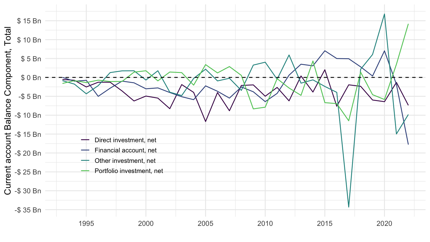

Hungary

MEI_BOP6 %>%
  filter(LOCATION %in% c("HUN"),
         # B6BLTT01: Current account, balance
         # B6BLPI01: Primary income, balance
         # B6BLSI01: Secondary income, balance
         SUBJECT %in% c("B6FADI01", "B6FAPI10", "B6FAOI01", "B6FATT01"),
         # CXCU: US Dollars, sum over component sub-periods, s.a
         MEASURE == "CXCU",
         FREQUENCY == "A") %>%
  year_to_date %>%
  left_join(MEI_BOP6_var$SUBJECT, by = "SUBJECT") %>%
  group_by(LOCATION) %>%
  ggplot(.) + xlab("") + ylab("Current account Balance Component, Total") + 
  geom_line(aes(x = date, y = obsValue/10^3, color = Subject)) + 
  theme_minimal() + scale_color_manual(values = viridis(5)[1:4]) +
  theme(legend.title = element_blank(),
        legend.position = c(0.2, 0.9),
        legend.text = element_text(size = 8),
        legend.key.size = unit(0.9, 'lines')) +
  scale_x_date(breaks = seq(1950, 2100, 5) %>% paste0("-01-01") %>% as.Date,
               labels = date_format("%Y")) +
  scale_y_continuous(breaks = seq(-20000, 400000, 5),
                     labels = dollar_format(accuracy = 1, suffix = " Bn", prefix = "$ ")) +
  geom_hline(yintercept = 0, linetype = "dashed", color = "black")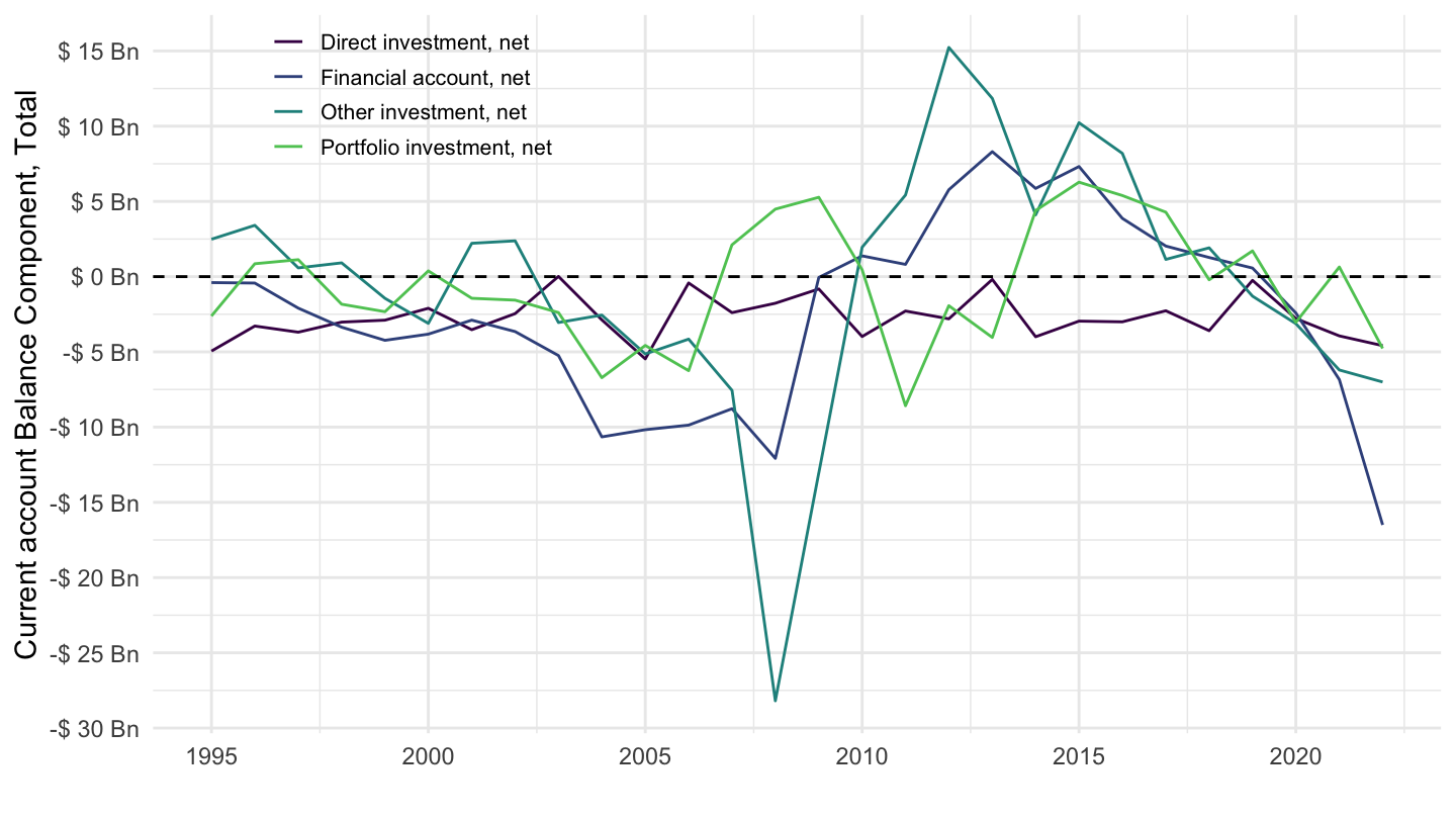

Portugal

MEI_BOP6 %>%
  filter(LOCATION %in% c("PRT"),
         # B6BLTT01: Current account, balance
         # B6BLPI01: Primary income, balance
         # B6BLSI01: Secondary income, balance
         SUBJECT %in% c("B6FADI01", "B6FAPI10", "B6FAOI01", "B6FATT01"),
         # CXCU: US Dollars, sum over component sub-periods, s.a
         MEASURE == "CXCU",
         FREQUENCY == "A") %>%
  year_to_date %>%
  left_join(MEI_BOP6_var$SUBJECT, by = "SUBJECT") %>%
  group_by(LOCATION) %>%
  ggplot(.) + xlab("") + ylab("Current account Balance Component, Total") + 
  geom_line(aes(x = date, y = obsValue/10^3, color = Subject)) + 
  theme_minimal() + scale_color_manual(values = viridis(5)[1:4]) +
  theme(legend.title = element_blank(),
        legend.position = c(0.2, 0.9),
        legend.text = element_text(size = 8),
        legend.key.size = unit(0.9, 'lines')) +
  scale_x_date(breaks = seq(1950, 2100, 2) %>% paste0("-01-01") %>% as.Date,
               labels = date_format("%Y")) +
  scale_y_continuous(breaks = seq(-20000, 400000, 5),
                     labels = dollar_format(accuracy = 1, suffix = " Bn", prefix = "$ ")) +
  geom_hline(yintercept = 0, linetype = "dashed", color = "black")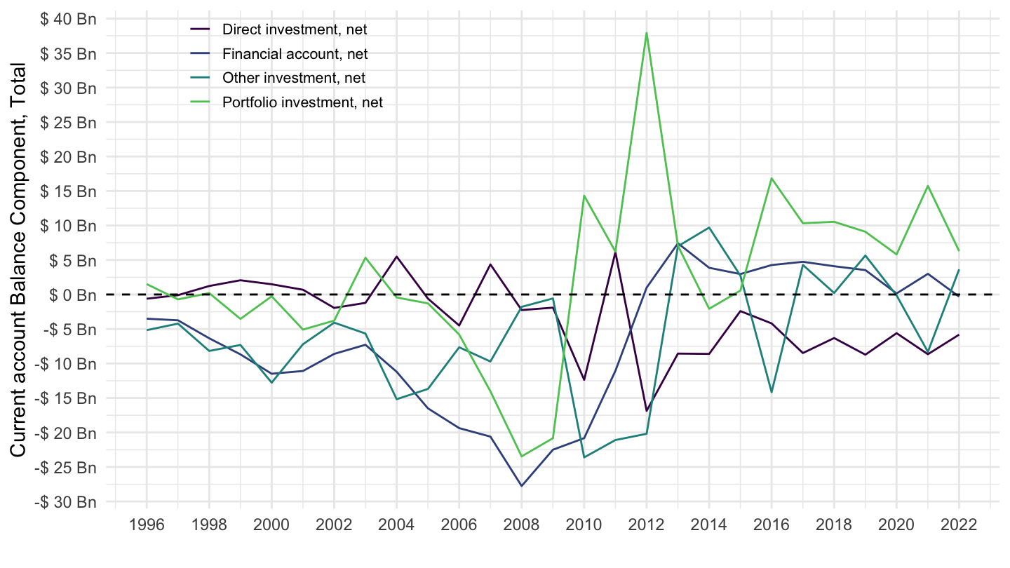

Austria

MEI_BOP6 %>%
  filter(LOCATION %in% c("AUT"),
         # B6BLTT01: Current account, balance
         # B6BLPI01: Primary income, balance
         # B6BLSI01: Secondary income, balance
         SUBJECT %in% c("B6FADI01", "B6FAPI10", "B6FAOI01", "B6FATT01"),
         # CXCU: US Dollars, sum over component sub-periods, s.a
         MEASURE == "CXCU",
         FREQUENCY == "A") %>%
  year_to_date %>%
  left_join(MEI_BOP6_var$SUBJECT, by = "SUBJECT") %>%
  group_by(LOCATION) %>%
  ggplot(.) + xlab("") + ylab("Current account Balance Component, Total") + 
  geom_line(aes(x = date, y = obsValue/10^3, color = Subject)) + 
  theme_minimal() + scale_color_manual(values = viridis(5)[1:4]) +
  theme(legend.title = element_blank(),
        legend.position = c(0.2, 0.8),
        legend.text = element_text(size = 8),
        legend.key.size = unit(0.9, 'lines')) +
  scale_x_date(breaks = seq(1950, 2100, 2) %>% paste0("-01-01") %>% as.Date,
               labels = date_format("%Y")) +
  scale_y_continuous(breaks = seq(-20000, 400000, 5),
                     labels = dollar_format(accuracy = 1, suffix = " Bn", prefix = "$ ")) +
  geom_hline(yintercept = 0, linetype = "dashed", color = "black")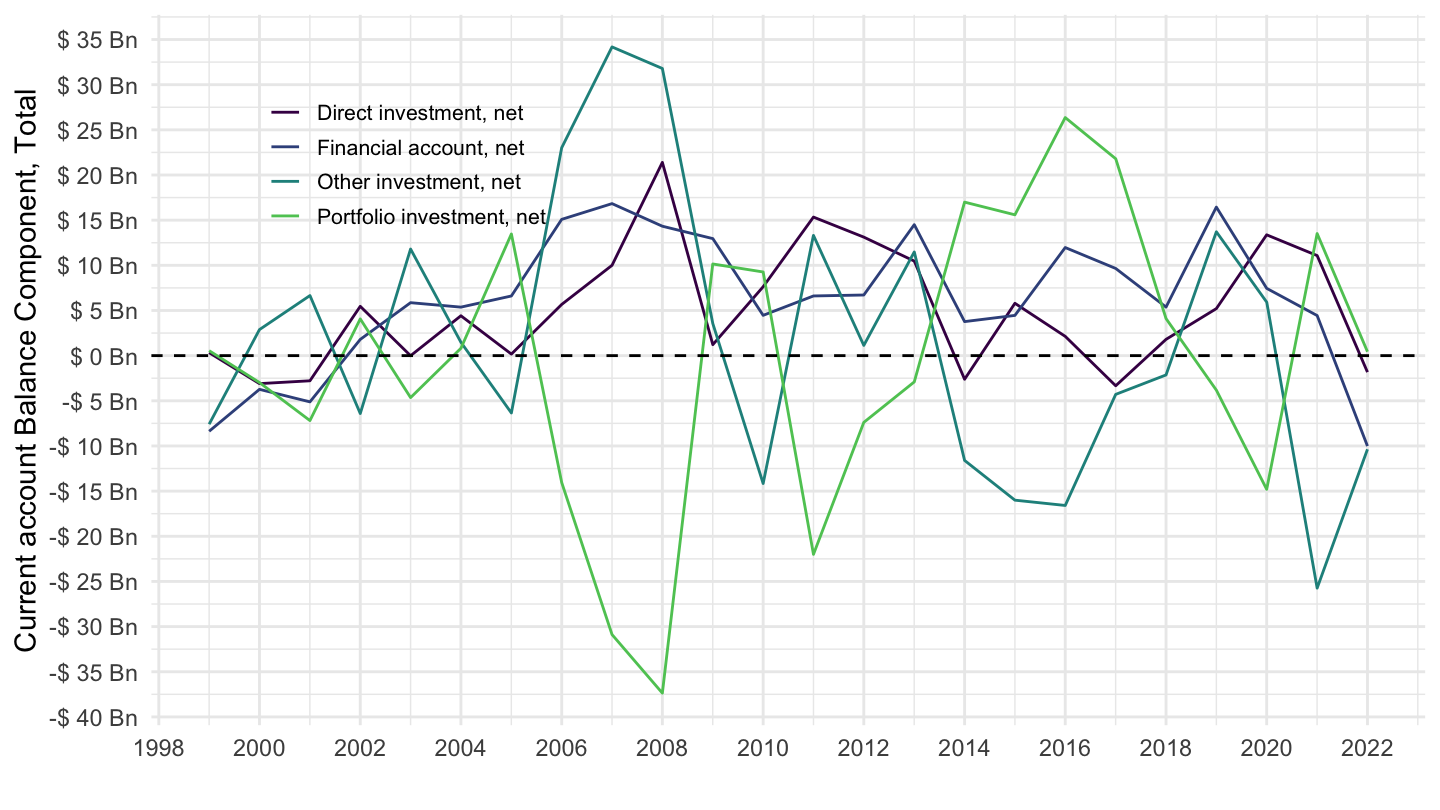

Current Account Decompositions

Germany

MEI_BOP6 %>%
  filter(LOCATION %in% c("DEU"),
         # B6BLTT01: Current account, balance
         # B6BLPI01: Primary income, balance
         # B6BLSI01: Secondary income, balance
         SUBJECT %in% c("B6BLPI01", "B6BLSI01", "B6BLTD01", "B6BLSE01"),
         # CXCUSA: US Dollars, sum over component sub-periods, s.a
         MEASURE == "CXCUSA",
         FREQUENCY == "Q") %>%
  quarter_to_date %>%
  left_join(MEI_BOP6_var$SUBJECT, by = "SUBJECT") %>%
  group_by(LOCATION) %>%
  ggplot(.) + xlab("") + ylab("Current account Balance Component, Total") + 
  geom_line(aes(x = date, y = obsValue/10^3, color = Subject)) + 
  theme_minimal() + scale_color_manual(values = viridis(5)[1:4]) +
  theme(legend.title = element_blank(),
        legend.position = c(0.2, 0.8),
        legend.text = element_text(size = 8),
        legend.key.size = unit(0.9, 'lines')) +
  scale_x_date(breaks = seq(1950, 2100, 5) %>% paste0("-01-01") %>% as.Date,
               labels = date_format("%Y")) +
  scale_y_continuous(breaks = seq(-20000, 400000, 10),
                     labels = dollar_format(accuracy = 1, suffix = " Bn", prefix = "$ ")) +
  geom_hline(yintercept = 0, linetype = "dashed", color = "black")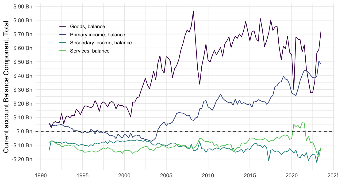

Euro Area

MEI_BOP6 %>%
  filter(LOCATION %in% c("EA20"),
         # B6BLTT01: Current account, balance
         # B6BLPI01: Primary income, balance
         # B6BLSI01: Secondary income, balance
         SUBJECT %in% c("B6BLPI01", "B6BLSI01", "B6BLTD01", "B6BLSE01"),
         # CXCUSA: US Dollars, sum over component sub-periods, s.a
         MEASURE == "CXCUSA",
         FREQUENCY == "Q") %>%
  quarter_to_date %>%
  left_join(MEI_BOP6_var$SUBJECT, by = "SUBJECT") %>%
  group_by(LOCATION) %>%
  ggplot(.) + xlab("") + ylab("Current account Balance Component, Total") + 
  geom_line(aes(x = date, y = obsValue/10^3, color = Subject)) + 
  theme_minimal() + scale_color_manual(values = viridis(5)[1:4]) +
  theme(legend.title = element_blank(),
        legend.position = c(0.2, 0.8),
        legend.text = element_text(size = 8),
        legend.key.size = unit(0.9, 'lines')) +
  scale_x_date(breaks = seq(1950, 2100, 2) %>% paste0("-01-01") %>% as.Date,
               labels = date_format("%Y")) +
  scale_y_continuous(breaks = seq(-20000, 400000, 20),
                     labels = dollar_format(accuracy = 1, suffix = " Bn", prefix = "$ ")) +
  geom_hline(yintercept = 0, linetype = "dashed", color = "black")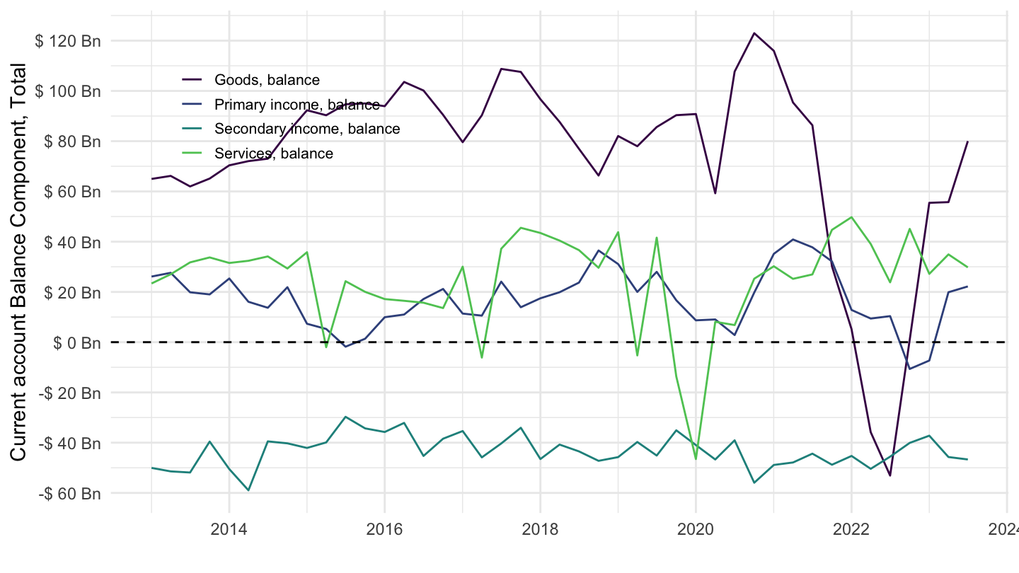

China

MEI_BOP6 %>%
  filter(LOCATION %in% c("CHN"),
         # B6BLTT01: Current account, balance
         # B6BLPI01: Primary income, balance
         # B6BLSI01: Secondary income, balance
         SUBJECT %in% c("B6BLPI01", "B6BLSI01", "B6BLTD01", "B6BLSE01"),
         # CXCUSA: US Dollars, sum over component sub-periods, s.a
         MEASURE == "CXCUSA",
         FREQUENCY == "Q") %>%
  quarter_to_date %>%
  left_join(MEI_BOP6_var$SUBJECT, by = "SUBJECT") %>%
  group_by(LOCATION) %>%
  ggplot(.) + xlab("") + ylab("Current account Balance Component, Total") + 
  geom_line(aes(x = date, y = obsValue/10^3, color = Subject)) + 
  theme_minimal() + scale_color_manual(values = viridis(5)[1:4]) +
  theme(legend.title = element_blank(),
        legend.position = c(0.2, 0.8),
        legend.text = element_text(size = 8),
        legend.key.size = unit(0.9, 'lines')) +
  scale_x_date(breaks = seq(1950, 2100, 5) %>% paste0("-01-01") %>% as.Date,
               labels = date_format("%Y")) +
  scale_y_continuous(breaks = seq(-20000, 400000, 50),
                     labels = dollar_format(accuracy = 1, suffix = " Bn", prefix = "$ ")) +
  geom_hline(yintercept = 0, linetype = "dashed", color = "black")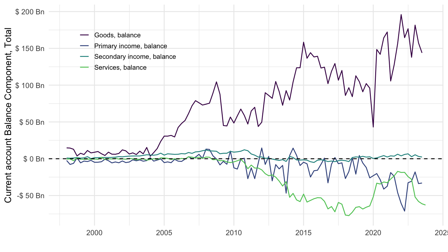

United Kingdom

MEI_BOP6 %>%
  filter(LOCATION %in% c("GBR"),
         # B6BLTT01: Current account, balance
         # B6BLPI01: Primary income, balance
         # B6BLSI01: Secondary income, balance
         SUBJECT %in% c("B6BLPI01", "B6BLSI01", "B6BLTD01", "B6BLSE01"),
         # CXCUSA: US Dollars, sum over component sub-periods, s.a
         MEASURE == "CXCUSA",
         FREQUENCY == "Q") %>%
  quarter_to_date %>%
  left_join(MEI_BOP6_var$SUBJECT, by = "SUBJECT") %>%
  group_by(LOCATION) %>%
  ggplot(.) + xlab("") + ylab("Current account Balance Component, Total") + 
  geom_line(aes(x = date, y = obsValue/10^3, color = Subject)) + 
  theme_minimal() + scale_color_manual(values = viridis(5)[1:4]) +
  theme(legend.title = element_blank(),
        legend.position = c(0.2, 0.8),
        legend.text = element_text(size = 8),
        legend.key.size = unit(0.9, 'lines')) +
  scale_x_date(breaks = seq(1950, 2100, 5) %>% paste0("-01-01") %>% as.Date,
               labels = date_format("%Y")) +
  scale_y_continuous(breaks = seq(-20000, 400000, 10),
                     labels = dollar_format(accuracy = 1, suffix = " Bn", prefix = "$ ")) +
  geom_hline(yintercept = 0, linetype = "dashed", color = "black")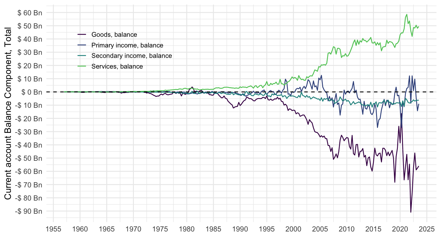

South Korea

MEI_BOP6 %>%
  filter(LOCATION %in% c("KOR"),
         # B6BLTT01: Current account, balance
         # B6BLPI01: Primary income, balance
         # B6BLSI01: Secondary income, balance
         SUBJECT %in% c("B6BLPI01", "B6BLSI01", "B6BLTD01", "B6BLSE01"),
         # CXCUSA: US Dollars, sum over component sub-periods, s.a
         MEASURE == "CXCUSA",
         FREQUENCY == "Q") %>%
  quarter_to_date %>%
  left_join(MEI_BOP6_var$SUBJECT, by = "SUBJECT") %>%
  group_by(LOCATION) %>%
  ggplot(.) + xlab("") + ylab("Current account Balance Component, Total") + 
  geom_line(aes(x = date, y = obsValue/10^3, color = Subject)) + 
  theme_minimal() + scale_color_manual(values = viridis(5)[1:4]) +
  theme(legend.title = element_blank(),
        legend.position = c(0.2, 0.8),
        legend.text = element_text(size = 8),
        legend.key.size = unit(0.9, 'lines')) +
  scale_x_date(breaks = seq(1950, 2100, 5) %>% paste0("-01-01") %>% as.Date,
               labels = date_format("%Y")) +
  scale_y_continuous(breaks = seq(-20000, 400000, 10),
                     labels = dollar_format(accuracy = 1, suffix = " Bn", prefix = "$ ")) +
  geom_hline(yintercept = 0, linetype = "dashed", color = "black")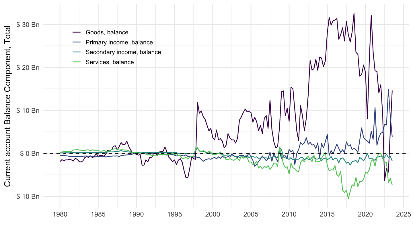

Sweden

MEI_BOP6 %>%
  filter(LOCATION %in% c("SWE"),
         # B6BLTT01: Current account, balance
         # B6BLPI01: Primary income, balance
         # B6BLSI01: Secondary income, balance
         SUBJECT %in% c("B6BLPI01", "B6BLSI01", "B6BLTD01", "B6BLSE01"),
         # CXCUSA: US Dollars, sum over component sub-periods, s.a
         MEASURE == "CXCUSA",
         FREQUENCY == "Q") %>%
  quarter_to_date %>%
  left_join(MEI_BOP6_var$SUBJECT, by = "SUBJECT") %>%
  group_by(LOCATION) %>%
  ggplot(.) + xlab("") + ylab("Current account Balance Component, Total") + 
  geom_line(aes(x = date, y = obsValue/10^3, color = Subject)) + 
  theme_minimal() + scale_color_manual(values = viridis(5)[1:4]) +
  theme(legend.title = element_blank(),
        legend.position = c(0.2, 0.8),
        legend.text = element_text(size = 8),
        legend.key.size = unit(0.9, 'lines')) +
  scale_x_date(breaks = seq(1950, 2100, 5) %>% paste0("-01-01") %>% as.Date,
               labels = date_format("%Y")) +
  scale_y_continuous(breaks = seq(-20000, 400000, 1),
                     labels = dollar_format(accuracy = 1, suffix = " Bn", prefix = "$ ")) +
  geom_hline(yintercept = 0, linetype = "dashed", color = "black")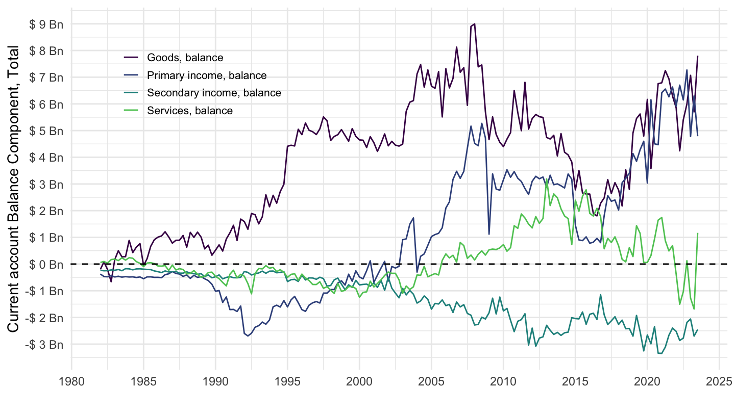

New Zealand

MEI_BOP6 %>%
  filter(LOCATION %in% c("NZL"),
         # B6BLTT01: Current account, balance
         # B6BLPI01: Primary income, balance
         # B6BLSI01: Secondary income, balance
         SUBJECT %in% c("B6BLPI01", "B6BLSI01", "B6BLTD01", "B6BLSE01"),
         # CXCUSA: US Dollars, sum over component sub-periods, s.a
         MEASURE == "CXCUSA",
         FREQUENCY == "Q") %>%
  quarter_to_date %>%
  left_join(MEI_BOP6_var$SUBJECT, by = "SUBJECT") %>%
  group_by(LOCATION) %>%
  ggplot(.) + xlab("") + ylab("Current account Balance Component, Total") + 
  geom_line(aes(x = date, y = obsValue/10^3, color = Subject)) + 
  theme_minimal() + scale_color_manual(values = viridis(5)[1:4]) +
  theme(legend.title = element_blank(),
        legend.position = c(0.2, 0.2),
        legend.text = element_text(size = 8),
        legend.key.size = unit(0.9, 'lines')) +
  scale_x_date(breaks = seq(1950, 2100, 5) %>% paste0("-01-01") %>% as.Date,
               labels = date_format("%Y")) +
  scale_y_continuous(breaks = seq(-20000, 400000, 1),
                     labels = dollar_format(accuracy = 1, suffix = " Bn", prefix = "$ ")) +
  geom_hline(yintercept = 0, linetype = "dashed", color = "black")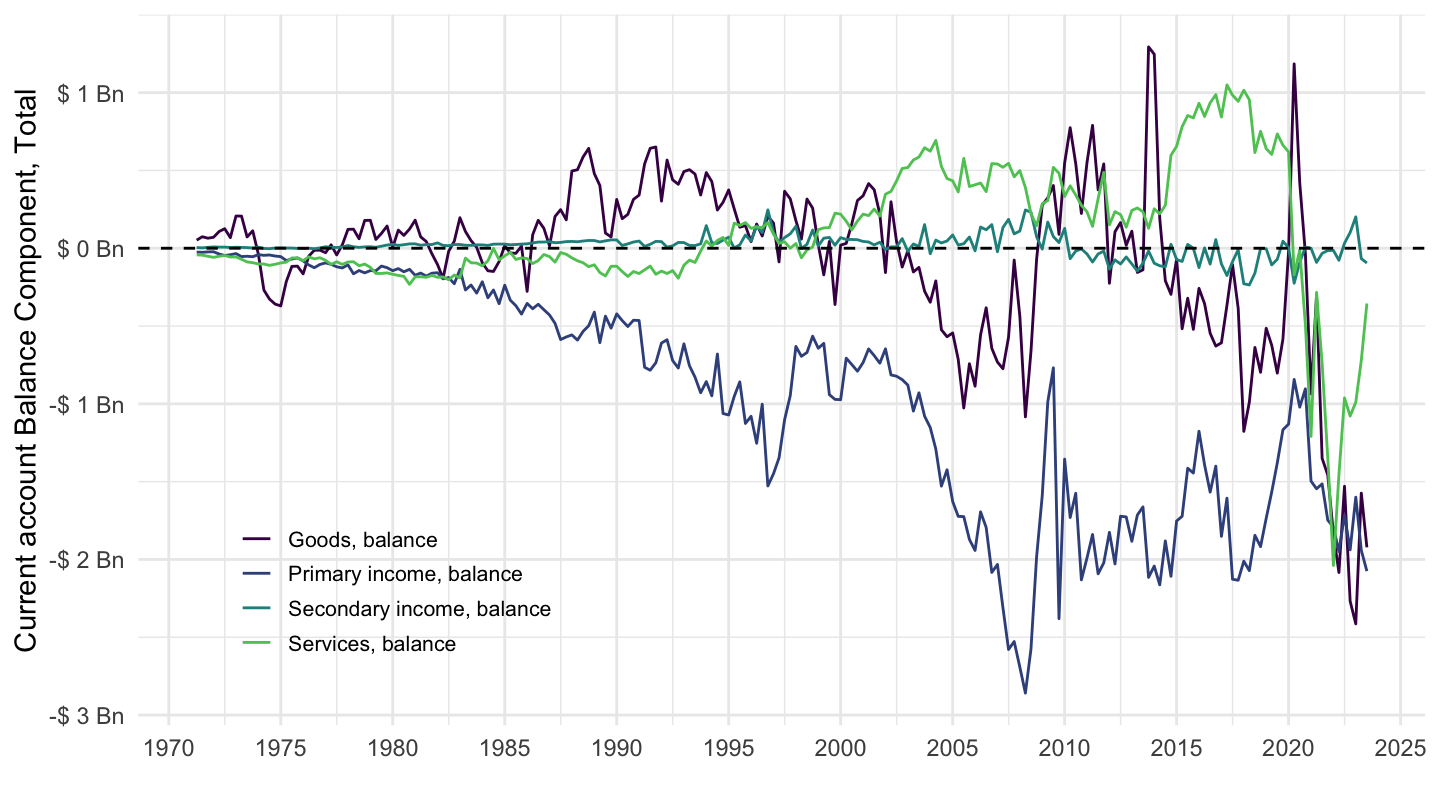

Canada

MEI_BOP6 %>%
  filter(LOCATION %in% c("CAN"),
         # B6BLTT01: Current account, balance
         # B6BLPI01: Primary income, balance
         # B6BLSI01: Secondary income, balance
         SUBJECT %in% c("B6BLPI01", "B6BLSI01", "B6BLTD01", "B6BLSE01"),
         # CXCUSA: US Dollars, sum over component sub-periods, s.a
         MEASURE == "CXCUSA",
         FREQUENCY == "Q") %>%
  quarter_to_date %>%
  left_join(MEI_BOP6_var$SUBJECT, by = "SUBJECT") %>%
  group_by(LOCATION) %>%
  ggplot(.) + xlab("") + ylab("Current account Balance Component, Total") + 
  geom_line(aes(x = date, y = obsValue/10^3, color = Subject)) + 
  theme_minimal() + scale_color_manual(values = viridis(5)[1:4]) +
  theme(legend.title = element_blank(),
        legend.position = c(0.2, 0.8),
        legend.text = element_text(size = 8),
        legend.key.size = unit(0.9, 'lines')) +
  scale_x_date(breaks = seq(1950, 2100, 5) %>% paste0("-01-01") %>% as.Date,
               labels = date_format("%Y")) +
  scale_y_continuous(breaks = seq(-20000, 400000, 5),
                     labels = dollar_format(accuracy = 1, suffix = " Bn", prefix = "$ ")) +
  geom_hline(yintercept = 0, linetype = "dashed", color = "black")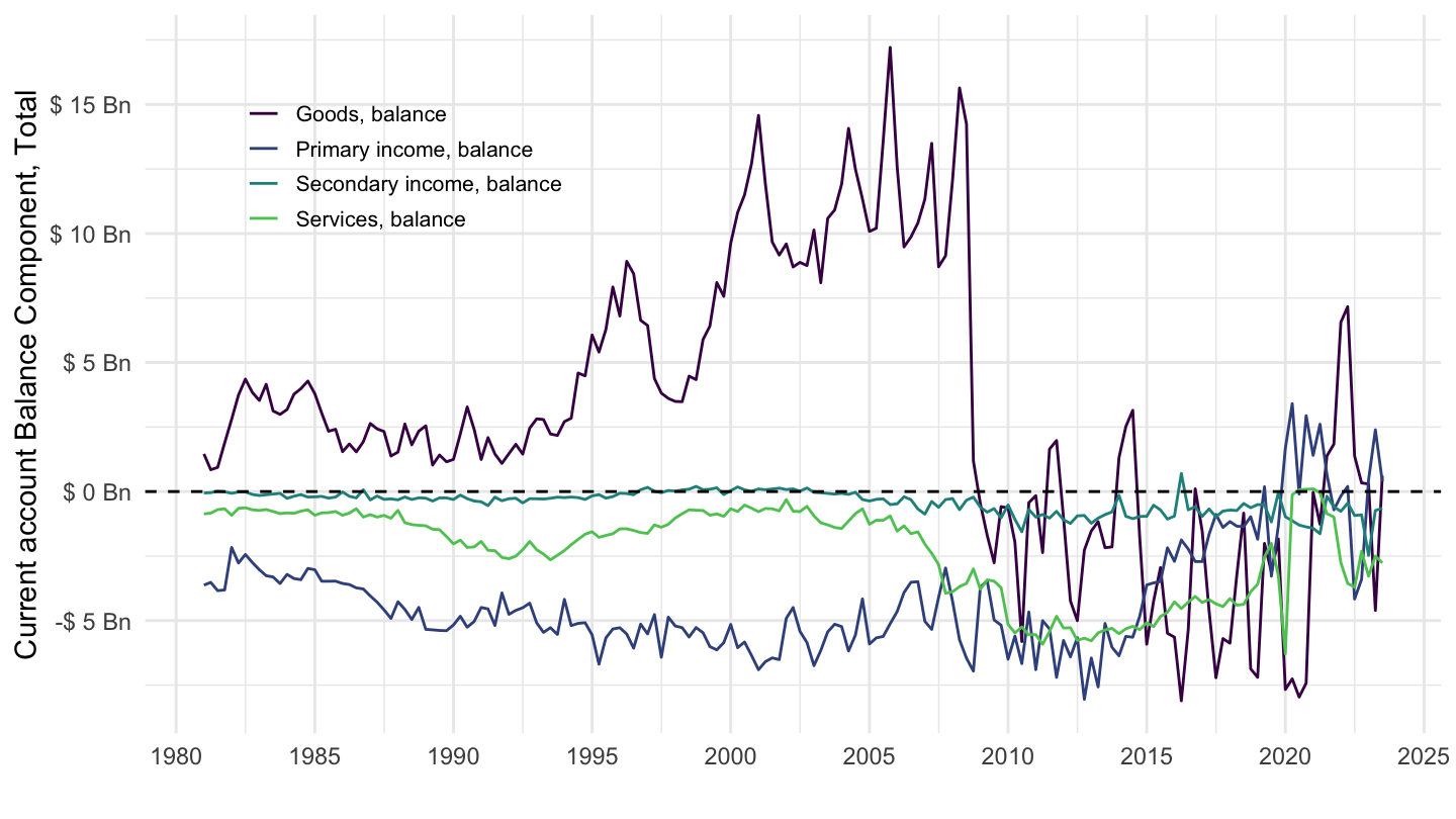

Australia

All

MEI_BOP6 %>%
  filter(LOCATION %in% c("AUS"),
         # B6BLTT01: Current account, balance
         # B6BLPI01: Primary income, balance
         # B6BLSI01: Secondary income, balance
         SUBJECT %in% c("B6BLPI01", "B6BLSI01", "B6BLTD01", "B6BLSE01"),
         # CXCUSA: US Dollars, sum over component sub-periods, s.a
         MEASURE == "CXCUSA",
         FREQUENCY == "Q") %>%
  quarter_to_date %>%
  left_join(MEI_BOP6_var$SUBJECT, by = "SUBJECT") %>%
  group_by(LOCATION) %>%
  ggplot(.) + xlab("") + ylab("Current account Balance Component, Total") + 
  geom_line(aes(x = date, y = obsValue/10^3, color = Subject)) + 
  theme_minimal() + scale_color_manual(values = viridis(5)[1:4]) +
  theme(legend.title = element_blank(),
        legend.position = c(0.2, 0.8),
        legend.text = element_text(size = 8),
        legend.key.size = unit(0.9, 'lines')) +
  scale_x_date(breaks = seq(1950, 2100, 5) %>% paste0("-01-01") %>% as.Date,
               labels = date_format("%Y")) +
  scale_y_continuous(breaks = seq(-20000, 400000, 10),
                     labels = dollar_format(accuracy = 1, suffix = " Bn", prefix = "$ ")) +
  geom_hline(yintercept = 0, linetype = "dashed", color = "black")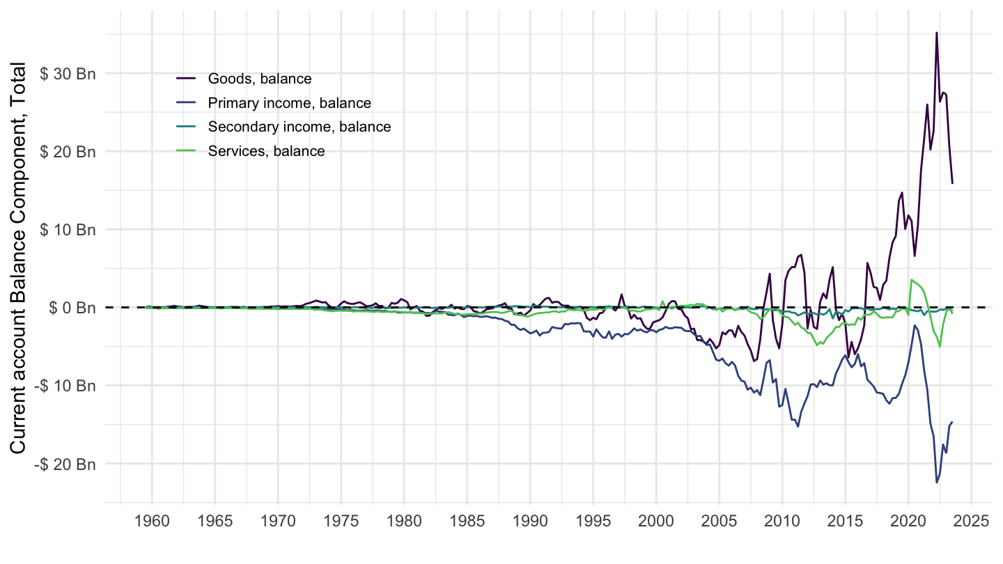

2010

MEI_BOP6 %>%
  filter(LOCATION %in% c("AUS"),
         # B6BLTT01: Current account, balance
         # B6BLPI01: Primary income, balance
         # B6BLSI01: Secondary income, balance
         SUBJECT %in% c("B6BLPI01", "B6BLSI01", "B6BLTD01", "B6BLSE01"),
         # CXCUSA: US Dollars, sum over component sub-periods, s.a
         MEASURE == "CXCUSA",
         FREQUENCY == "Q") %>%
  quarter_to_date %>%
  filter(date >= as.Date("2010-01-01")) %>%
  left_join(MEI_BOP6_var$SUBJECT, by = "SUBJECT") %>%
  group_by(LOCATION) %>%
  ggplot(.) + xlab("") + ylab("Current account Balance Component, Total") + 
  geom_line(aes(x = date, y = obsValue/10^3, color = Subject)) + 
  theme_minimal() + scale_color_manual(values = viridis(5)[1:4]) +
  theme(legend.title = element_blank(),
        legend.position = c(0.2, 0.9),
        legend.text = element_text(size = 8),
        legend.key.size = unit(0.9, 'lines')) +
  scale_x_date(breaks = seq(1950, 2100, 1) %>% paste0("-01-01") %>% as.Date,
               labels = date_format("%Y")) +
  scale_y_continuous(breaks = seq(-20000, 400000, 5),
                     labels = dollar_format(accuracy = 1, suffix = " Bn", prefix = "$ ")) +
  geom_hline(yintercept = 0, linetype = "dashed", color = "black")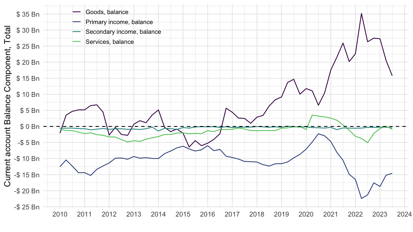

France

MEI_BOP6 %>%
  filter(LOCATION %in% c("FRA"),
         # B6BLTT01: Current account, balance
         # B6BLPI01: Primary income, balance
         # B6BLSI01: Secondary income, balance
         SUBJECT %in% c("B6BLPI01", "B6BLSI01", "B6BLTD01", "B6BLSE01"),
         # CXCUSA: US Dollars, sum over component sub-periods, s.a
         MEASURE == "CXCUSA",
         FREQUENCY == "Q") %>%
  quarter_to_date %>%
  left_join(MEI_BOP6_var$SUBJECT, by = "SUBJECT") %>%
  ggplot(.) + xlab("") + ylab("Current account Balance Component, Total") + 
  geom_line(aes(x = date, y = obsValue/10^3, color = Subject)) + 
  theme_minimal() + scale_color_manual(values = viridis(5)[1:4]) +
  theme(legend.title = element_blank(),
        legend.position = c(0.2, 0.9),
        legend.text = element_text(size = 8),
        legend.key.size = unit(0.9, 'lines')) +
  scale_x_date(breaks = seq(1950, 2100, 2) %>% paste0("-01-01") %>% as.Date,
               labels = date_format("%Y")) +
  scale_y_continuous(breaks = seq(-20000, 400000, 5),
                     labels = dollar_format(accuracy = 1, suffix = " Bn", prefix = "$ ")) +
  geom_hline(yintercept = 0, linetype = "dashed", color = "black")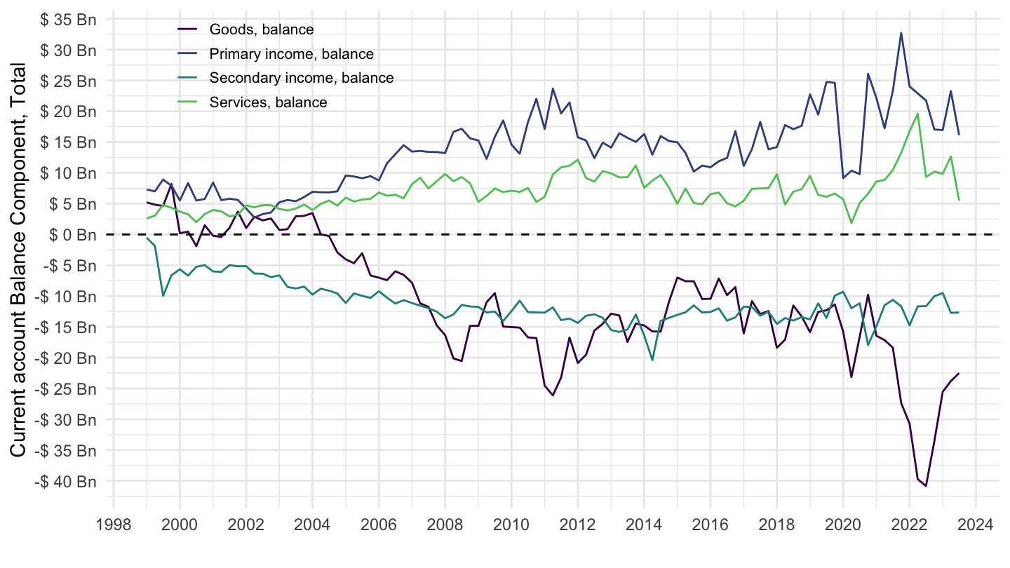

United States

MEI_BOP6 %>%
  filter(LOCATION %in% c("USA"),
         # B6BLTT01: Current account, balance
         # B6BLPI01: Primary income, balance
         # B6BLSI01: Secondary income, balance
         SUBJECT %in% c("B6BLPI01", "B6BLSI01", "B6BLTD01", "B6BLSE01"),
         # CXCUSA: US Dollars, sum over component sub-periods, s.a
         MEASURE == "CXCUSA",
         FREQUENCY == "Q") %>%
  quarter_to_date %>%
  left_join(MEI_BOP6_var$SUBJECT, by = "SUBJECT") %>%
  group_by(LOCATION) %>%
  ggplot(.) + xlab("") + ylab("Current account Balance Component, Total") + 
  geom_line(aes(x = date, y = obsValue/10^3, color = Subject)) + 
  theme_minimal() + scale_color_manual(values = viridis(5)[1:4]) +
  theme(legend.title = element_blank(),
        legend.position = c(0.2, 0.3),
        legend.text = element_text(size = 8),
        legend.key.size = unit(0.9, 'lines')) +
  scale_x_date(breaks = seq(1950, 2100, 5) %>% paste0("-01-01") %>% as.Date,
               labels = date_format("%Y")) +
  scale_y_continuous(breaks = seq(-20000, 400000, 20),
                     labels = dollar_format(accuracy = 1, suffix = " Bn", prefix = "$ ")) +
  geom_hline(yintercept = 0, linetype = "dashed", color = "black")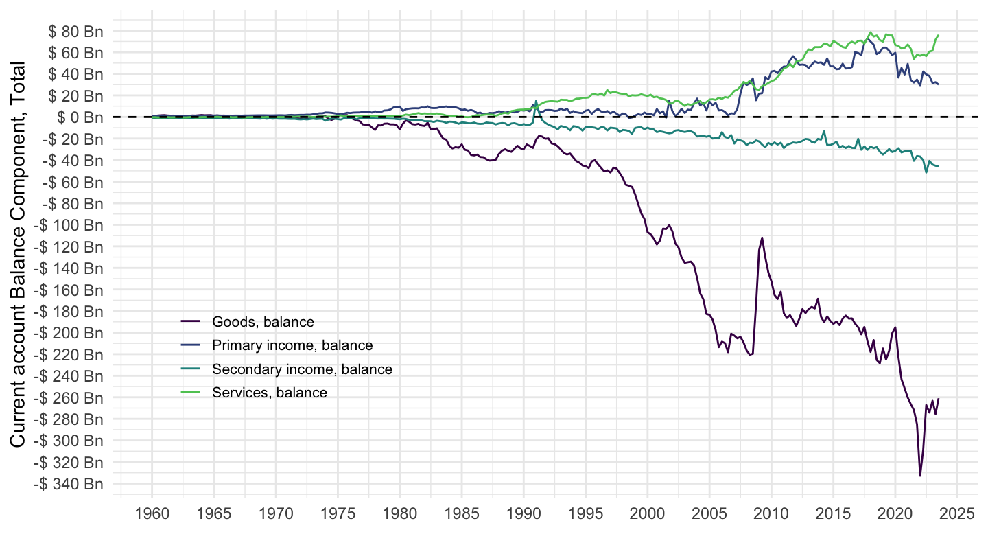

Poland

MEI_BOP6 %>%
  filter(LOCATION %in% c("POL"),
         # B6BLTT01: Current account, balance
         # B6BLPI01: Primary income, balance
         # B6BLSI01: Secondary income, balance
         SUBJECT %in% c("B6BLPI01", "B6BLSI01", "B6BLTD01", "B6BLSE01"),
         # CXCUSA: US Dollars, sum over component sub-periods, s.a
         MEASURE == "CXCUSA",
         FREQUENCY == "Q") %>%
  quarter_to_date %>%
  left_join(MEI_BOP6_var$SUBJECT, by = "SUBJECT") %>%
  group_by(LOCATION) %>%
  ggplot(.) + xlab("") + ylab("Current account Balance Component, Total") + 
  geom_line(aes(x = date, y = obsValue/10^3, color = Subject)) + 
  theme_minimal() + scale_color_manual(values = viridis(5)[1:4]) +
  theme(legend.title = element_blank(),
        legend.position = c(0.2, 0.9),
        legend.text = element_text(size = 8),
        legend.key.size = unit(0.9, 'lines')) +
  scale_x_date(breaks = seq(1950, 2100, 5) %>% paste0("-01-01") %>% as.Date,
               labels = date_format("%Y")) +
  scale_y_continuous(breaks = seq(-20000, 400000, 5),
                     labels = dollar_format(accuracy = 1, suffix = " Bn", prefix = "$ ")) +
  geom_hline(yintercept = 0, linetype = "dashed", color = "black")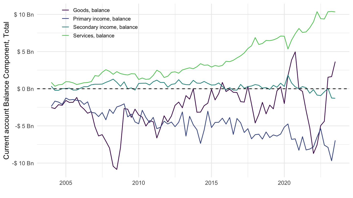

Czech Republic

MEI_BOP6 %>%
  filter(LOCATION %in% c("CZE"),
         # B6BLTT01: Current account, balance
         # B6BLPI01: Primary income, balance
         # B6BLSI01: Secondary income, balance
         SUBJECT %in% c("B6BLPI01", "B6BLSI01", "B6BLTD01", "B6BLSE01"),
         # CXCUSA: US Dollars, sum over component sub-periods, s.a
         MEASURE == "CXCUSA",
         FREQUENCY == "Q") %>%
  quarter_to_date %>%
  left_join(MEI_BOP6_var$SUBJECT, by = "SUBJECT") %>%
  group_by(LOCATION) %>%
  ggplot(.) + xlab("") + ylab("Current account Balance Component, Total") + 
  geom_line(aes(x = date, y = obsValue/10^3, color = Subject)) + 
  theme_minimal() + scale_color_manual(values = viridis(5)[1:4]) +
  theme(legend.title = element_blank(),
        legend.position = c(0.2, 0.3),
        legend.text = element_text(size = 8),
        legend.key.size = unit(0.9, 'lines')) +
  scale_x_date(breaks = seq(1950, 2100, 5) %>% paste0("-01-01") %>% as.Date,
               labels = date_format("%Y")) +
  scale_y_continuous(breaks = seq(-20000, 400000, 1),
                     labels = dollar_format(accuracy = 1, suffix = " Bn", prefix = "$ ")) +
  geom_hline(yintercept = 0, linetype = "dashed", color = "black")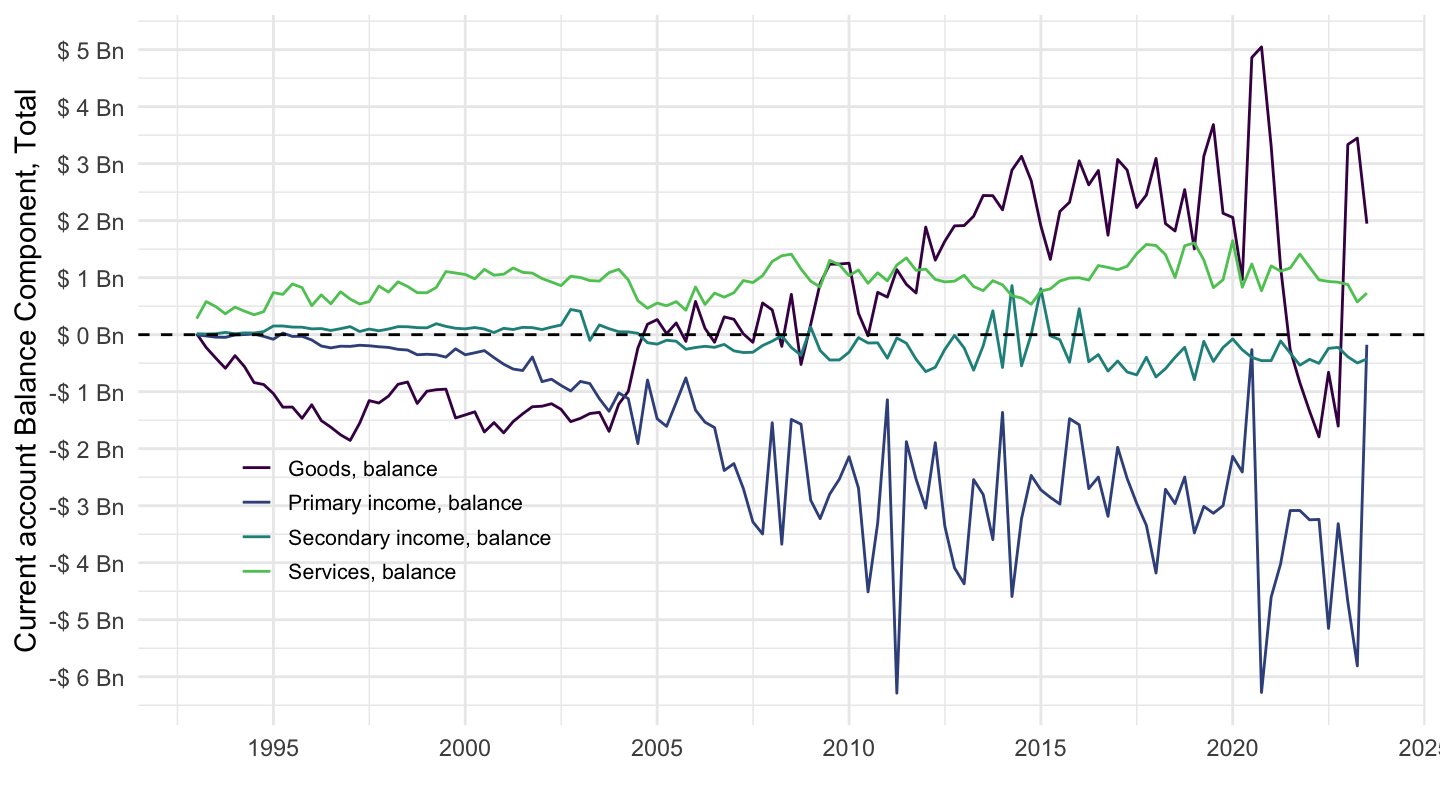

Hungary

MEI_BOP6 %>%
  filter(LOCATION %in% c("HUN"),
         # B6BLTT01: Current account, balance
         # B6BLPI01: Primary income, balance
         # B6BLSI01: Secondary income, balance
         SUBJECT %in% c("B6BLPI01", "B6BLSI01", "B6BLTD01", "B6BLSE01"),
         # CXCUSA: US Dollars, sum over component sub-periods, s.a
         MEASURE == "CXCUSA",
         FREQUENCY == "Q") %>%
  quarter_to_date %>%
  left_join(MEI_BOP6_var$SUBJECT, by = "SUBJECT") %>%
  group_by(LOCATION) %>%
  ggplot(.) + xlab("") + ylab("Current account Balance Component, Total") + 
  geom_line(aes(x = date, y = obsValue/10^3, color = Subject)) + 
  theme_minimal() + scale_color_manual(values = viridis(5)[1:4]) +
  theme(legend.title = element_blank(),
        legend.position = c(0.2, 0.9),
        legend.text = element_text(size = 8),
        legend.key.size = unit(0.9, 'lines')) +
  scale_x_date(breaks = seq(1950, 2100, 5) %>% paste0("-01-01") %>% as.Date,
               labels = date_format("%Y")) +
  scale_y_continuous(breaks = seq(-20000, 400000, 1),
                     labels = dollar_format(accuracy = 1, suffix = " Bn", prefix = "$ ")) +
  geom_hline(yintercept = 0, linetype = "dashed", color = "black")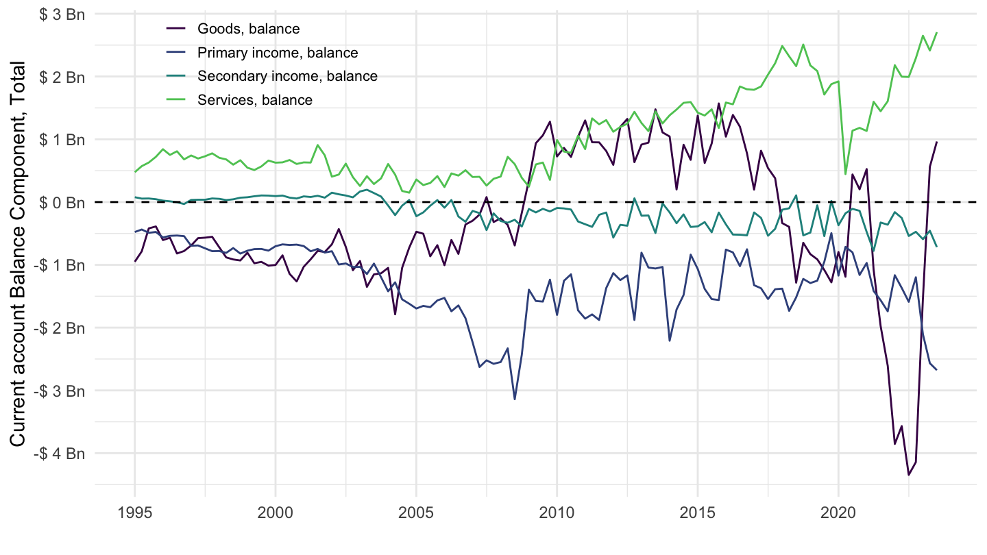

Portugal

MEI_BOP6 %>%
  filter(LOCATION %in% c("PRT"),
         # B6BLTT01: Current account, balance
         # B6BLPI01: Primary income, balance
         # B6BLSI01: Secondary income, balance
         SUBJECT %in% c("B6BLPI01", "B6BLSI01", "B6BLTD01", "B6BLSE01"),
         # CXCUSA: US Dollars, sum over component sub-periods, s.a
         MEASURE == "CXCUSA",
         FREQUENCY == "Q") %>%
  quarter_to_date %>%
  left_join(MEI_BOP6_var$SUBJECT, by = "SUBJECT") %>%
  group_by(LOCATION) %>%
  ggplot(.) + xlab("") + ylab("Current account Balance Component, Total") + 
  geom_line(aes(x = date, y = obsValue/10^3, color = Subject)) + 
  theme_minimal() + scale_color_manual(values = viridis(5)[1:4]) +
  theme(legend.title = element_blank(),
        legend.position = c(0.2, 0.9),
        legend.text = element_text(size = 8),
        legend.key.size = unit(0.9, 'lines')) +
  scale_x_date(breaks = seq(1950, 2100, 2) %>% paste0("-01-01") %>% as.Date,
               labels = date_format("%Y")) +
  scale_y_continuous(breaks = seq(-20000, 400000, 1),
                     labels = dollar_format(accuracy = 1, suffix = " Bn", prefix = "$ ")) +
  geom_hline(yintercept = 0, linetype = "dashed", color = "black")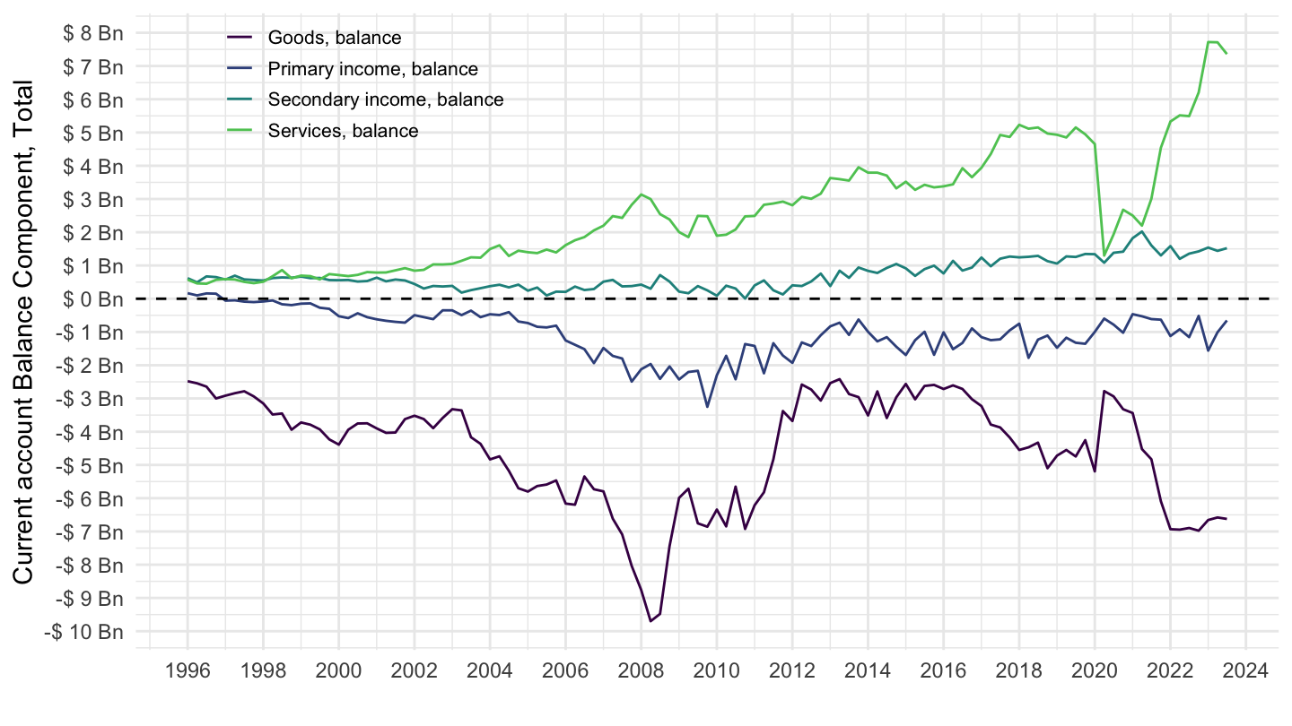

Austria

MEI_BOP6 %>%
  filter(LOCATION %in% c("AUT"),
         # B6BLTT01: Current account, balance
         # B6BLPI01: Primary income, balance
         # B6BLSI01: Secondary income, balance
         SUBJECT %in% c("B6BLPI01", "B6BLSI01", "B6BLTD01", "B6BLSE01"),
         # CXCUSA: US Dollars, sum over component sub-periods, s.a
         MEASURE == "CXCUSA",
         FREQUENCY == "Q") %>%
  quarter_to_date %>%
  left_join(MEI_BOP6_var$SUBJECT, by = "SUBJECT") %>%
  group_by(LOCATION) %>%
  ggplot(.) + xlab("") + ylab("Current account Balance Component, Total") + 
  geom_line(aes(x = date, y = obsValue/10^3, color = Subject)) + 
  theme_minimal() + scale_color_manual(values = viridis(5)[1:4]) +
  theme(legend.title = element_blank(),
        legend.position = c(0.2, 0.8),
        legend.text = element_text(size = 8),
        legend.key.size = unit(0.9, 'lines')) +
  scale_x_date(breaks = seq(1950, 2100, 2) %>% paste0("-01-01") %>% as.Date,
               labels = date_format("%Y")) +
  scale_y_continuous(breaks = seq(-20000, 400000, 1),
                     labels = dollar_format(accuracy = 1, suffix = " Bn", prefix = "$ ")) +
  geom_hline(yintercept = 0, linetype = "dashed", color = "black")

Balance of Payments BPM6 - MEI_BOP6

Data - OECD

François Geerolf

Info

LAST_DOWNLOAD

LAST_COMPILE

Last

Layout - By country

Nobs - Javascript

SUBJECT

All

China

MEASURE

FREQUENCY

LOCATION

obsTime

Example

CA (% of GDP)

US, Europe, France, Germany

1990-

1999-

Belgium, Greece, Netherlands

Annual

France and Germany

Annual

Quarterly

Netherlands, Denmark, Italy

Australia, Japan, Switzerland

Current Account Balance

France, Germany, Italy

Netherlands, Switzerland, Sweden

CA Decompositions - ALL

Germany

France

United States

Capital Account Decompositions

Germany

Euro Area

China

United Kingdom

South Korea

Sweden

New Zealand

Canada

Australia

All

2010

France

United States

Poland

Czech Republic

Hungary

Portugal

Austria

Capital Account Decompositions - Annual

Germany

Euro Area

China

United Kingdom

South Korea

Sweden

New Zealand

Canada

Australia

All

2010

France

United States

Poland

Czech Republic

Hungary

Portugal

Austria

Current Account Decompositions

Germany

Euro Area

China

United Kingdom

South Korea

Sweden