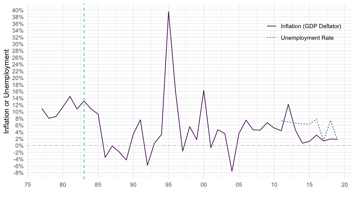
Last observation: 2027 (N = 783)
First observation: 1947 (N = 1)
Last data update: 01 août 2026, 21:45
Last compile: 04 oct. 2026, 22:44
UNE_DEAP_SEX_AGE_RT_A |>
  filter(sex == "SEX_T",
         classif1 == "AGE_AGGREGATE_YGE15") |>
  left_join(ref_area, by = "ref_area") |>
  group_by(ref_area, Ref_area) |>
  summarise(Nobs = n()) |>
  mutate(Flag = gsub(" ", "-", str_to_lower(Ref_area)),
         Flag = paste0('<img src="../../bib/flags/vsmall/', Flag, '.png" alt="Flag">')) |>
  select(Flag, everything()) %>%
{if (is_html_output()) datatable(., filter = 'top', rownames = F, escape = F) else .}UNE_DEAP_SEX_AGE_RT_A |>
left_join(classif1, by = "classif1") |>
group_by(classif1, Classif1) |>
summarise(Nobs = n()) |>
arrange(-Nobs) %>%
{if (is_html_output()) datatable(., filter = 'top', rownames = F) else .}UNE_DEAP_SEX_AGE_RT_A |>
left_join(source, by = "source") |>
group_by(source, Source) |>
summarise(Nobs = n()) |>
arrange(-Nobs) %>%
{if (is_html_output()) datatable(., filter = 'top', rownames = F) else .}UNE_DEAP_SEX_AGE_RT_A |>
left_join(sex, by = "sex") |>
group_by(sex, Sex) |>
summarise(Nobs = n()) |>
arrange(-Nobs) %>%
{if (is_html_output()) datatable(., filter = 'top', rownames = F) else .}UNE_DEAP_SEX_AGE_RT_A |>
filter(sex == "SEX_T",
classif1 == "AGE_AGGREGATE_YGE15") |>
left_join(ref_area, by = "ref_area") |>
mutate(obs_value = round(obs_value, 1)) |>
group_by(ref_area, Ref_area) |>
arrange(time) |>
summarise(Nobs = n(),
`Year 1` = first(time),
`Inflation 1` = first(obs_value),
`Year 2` = last(time),
`Inflation 2` = last(obs_value)) |>
arrange(-Nobs) |>
mutate(Flag = gsub(" ", "-", str_to_lower(Ref_area)),
Flag = paste0('<img src="../../bib/flags/vsmall/', Flag, '.png" alt="Flag">')) |>
select(Flag, everything()) %>%
{if (is_html_output()) datatable(., filter = 'top', rownames = F, escape = F) else .}UNE_DEAP_SEX_AGE_RT_A |>
filter(ref_area %in% c("USA", "JPN", "CAN"),
sex == "SEX_T",
classif1 == "AGE_AGGREGATE_YGE15") |>
left_join(ref_area, by = "ref_area") |>
year_to_enddate() |>
mutate(obs_value = obs_value/100) |>
add_flag_color("Ref_area") |>
ggplot() + geom_line() + theme_minimal() + scale_color_identity() + add_flags +
aes(x = date, y = obs_value, color = color) +
xlab("") + ylab("Unemployment rate") +
theme(legend.title = element_blank(),
legend.position = c(0.15, 0.85)) +
scale_x_date(breaks = seq(1900, 2100, 5) |> paste0("-01-01") |> as.Date(),
labels = date_format("%Y")) +
scale_y_continuous(breaks = 0.01*seq(-100, 10000, 2),
labels = percent_format(a = 1)) +
geom_hline(yintercept = 0, linetype = "dashed", color = "grey")
UNE_DEAP_SEX_AGE_RT_A |>
  filter(ref_area %in% c("FRA", "DEU", "ESP"),
         sex == "SEX_T",
         classif1 == "AGE_AGGREGATE_YGE15") |>
  left_join(ref_area, by = "ref_area") |>
  year_to_enddate() |>
  mutate(obs_value = obs_value/100) |>
  add_flag_color("Ref_area") |>
  ggplot() + geom_line() + theme_minimal() + scale_color_identity() + add_flags +
  aes(x = date, y = obs_value, color = color) +
  xlab("") + ylab("Unemployment rate") +
  theme(legend.title = element_blank(),
        legend.position = c(0.15, 0.85)) +
  scale_x_date(breaks = seq(1900, 2100, 5) |> paste0("-01-01") |> as.Date(),
               labels = date_format("%Y")) +
  scale_y_continuous(breaks = 0.01*seq(-100, 10000, 2),
                     labels = percent_format(a = 1)) +
  geom_hline(yintercept = 0, linetype = "dashed", color = "grey")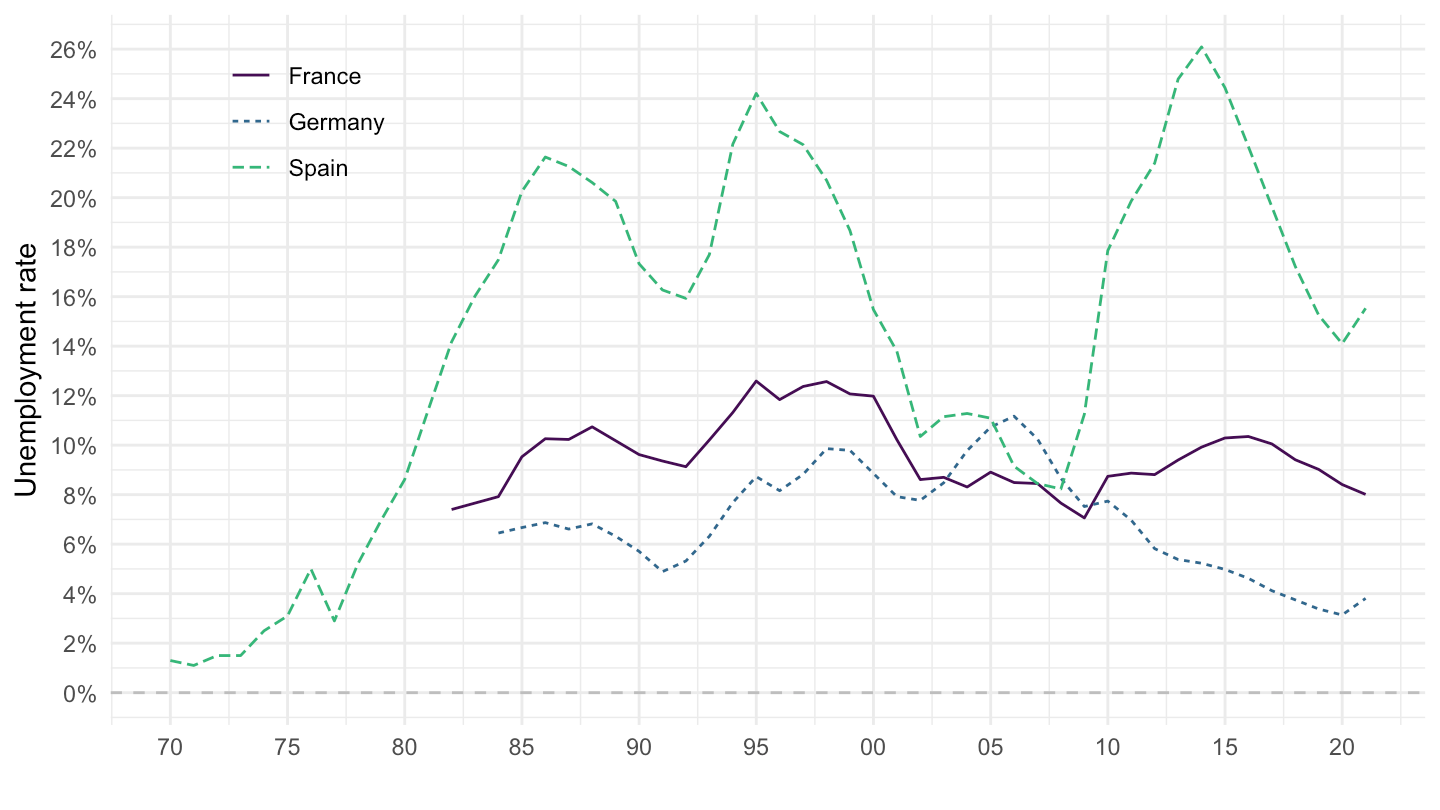
UNE_DEAP_SEX_AGE_RT_A |>
  filter(ref_area %in% c("HKG", "ITA", "KOR"),
         sex == "SEX_T",
         classif1 == "AGE_AGGREGATE_YGE15") |>
  left_join(ref_area, by = "ref_area") |>
  year_to_enddate() |>
  mutate(obs_value = obs_value/100) |>
  add_flag_color("Ref_area") |>
  ggplot() + geom_line() + theme_minimal() + scale_color_identity() + add_flags +
  aes(x = date, y = obs_value, color = color) +
  xlab("") + ylab("Unemployment rate") +
  theme(legend.title = element_blank(),
        legend.position = c(0.15, 0.85)) +
  scale_x_date(breaks = seq(1900, 2100, 5) |> paste0("-01-01") |> as.Date(),
               labels = date_format("%Y")) +
  scale_y_continuous(breaks = 0.01*seq(-100, 10000, 2),
                     labels = percent_format(a = 1)) +
  geom_hline(yintercept = 0, linetype = "dashed", color = "grey")
UNE_DEAP_SEX_AGE_RT_A |>
  filter(ref_area %in% c("HKG"),
         sex == "SEX_T",
         classif1 == "AGE_AGGREGATE_YGE15") |>
  mutate(date = paste0(time, "-12-31") |> as.Date()) |>
  select(date, value = obs_value) |>
  mutate(variable = "Unemployment Rate") |>
  bind_rows(NY.GDP.DEFL.KD.ZG |>
              filter(iso2c %in% c("HK")) |>
              mutate(date = paste0(year, "-12-31") |> as.Date()) |>
              select(date, value = value) |>
              mutate(variable = "Inflation (GDP Deflator)")) |>
  ggplot() + geom_line() + theme_minimal() +
  aes(x = date, y = value/100, color = variable, linetype = variable) +
  xlab("") + ylab("Hong Kong's Inflation or Unemployment") +
  scale_color_manual(values = viridis(4)[1:3]) +
  theme(legend.title = element_blank(),
        legend.position = c(0.85, 0.85)) +
  scale_x_date(breaks = seq(1900, 2100, 5) |> paste0("-01-01") |> as.Date(),
               labels = date_format("%Y")) +
  scale_y_continuous(breaks = 0.01*seq(-100, 10000, 2),
                     labels = percent_format(a = 1)) +
  geom_vline(xintercept = as.Date("1983-01-01"), linetype = "dashed", color = viridis(4)[3]) +
  geom_hline(yintercept = 0, linetype = "dashed", color = "black")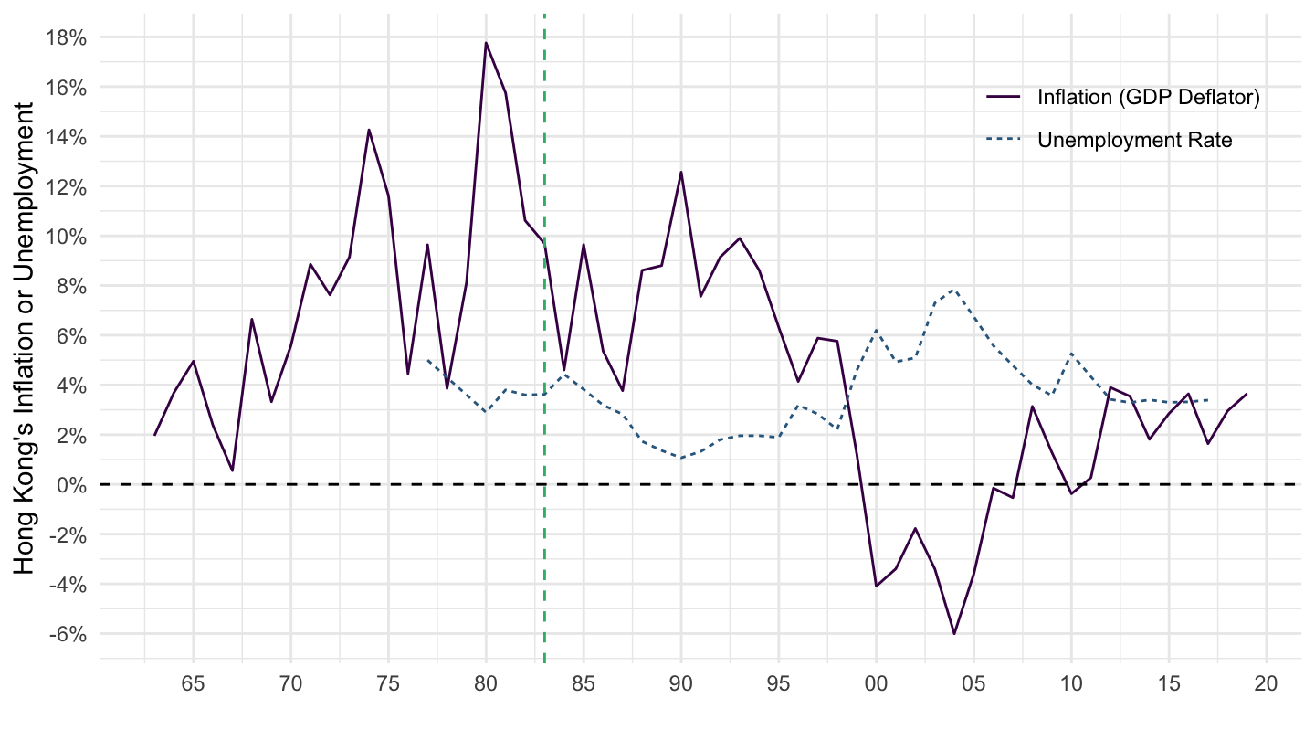
UNE_DEAP_SEX_AGE_RT_A |>
  filter(ref_area %in% c("HKG"),
         sex == "SEX_T",
         classif1 == "AGE_AGGREGATE_YGE15") |>
  mutate(date = paste0(time, "-12-31") |> as.Date()) |>
  select(date, value = obs_value) |>
  mutate(variable = "Unemployment Rate") |>
  bind_rows(NY.GDP.DEFL.KD.ZG |>
              filter(iso2c %in% c("HK")) |>
              mutate(date = paste0(year, "-12-31") |> as.Date()) |>
              select(date, value = value) |>
              mutate(variable = "Inflation (GDP Deflator)")) |>
  filter(date >= as.Date("1976-01-01")) |>
  ggplot() + geom_line() + theme_minimal() +
  aes(x = date, y = value/100, color = variable, linetype = variable) +
  xlab("") + ylab("Hong Kong's Inflation or Unemployment") +
  scale_color_manual(values = viridis(4)[1:3]) +
  theme(legend.title = element_blank(),
        legend.position = c(0.85, 0.85)) +
  scale_x_date(breaks = seq(1900, 2100, 5) |> paste0("-01-01") |> as.Date(),
               labels = date_format("%Y")) +
  scale_y_continuous(breaks = 0.01*seq(-100, 10000, 2),
                     labels = percent_format(a = 1)) +
  geom_vline(xintercept = as.Date("1983-01-01"), linetype = "dashed", color = viridis(4)[3]) +
  geom_hline(yintercept = 0, linetype = "dashed", color = "black")
UNE_DEAP_SEX_AGE_RT_A |>
  filter(ref_area %in% c("BEN"),
         sex == "SEX_T",
         classif1 == "AGE_AGGREGATE_YGE15") |>
  mutate(date = paste0(time, "-12-31") |> as.Date()) |>
  select(date, value = obs_value) |>
  mutate(variable = "Unemployment Rate") |>
  bind_rows(NY.GDP.DEFL.KD.ZG |>
              filter(iso2c %in% c("BJ")) |>
              mutate(date = paste0(year, "-12-31") |> as.Date()) |>
              select(date, value = value) |>
              mutate(variable = "Inflation (GDP Deflator)")) |>
  filter(date >= as.Date("1976-01-01")) |>
  ggplot() + geom_line() + theme_minimal() +
  aes(x = date, y = value/100, color = variable, linetype = variable) +
  xlab("") + ylab("Hong Kong's Inflation or Unemployment") +
  scale_color_manual(values = viridis(4)[1:3]) +
  theme(legend.title = element_blank(),
        legend.position = c(0.85, 0.85)) +
  scale_x_date(breaks = seq(1900, 2100, 5) |> paste0("-01-01") |> as.Date(),
               labels = date_format("%Y")) +
  scale_y_continuous(breaks = 0.01*seq(-100, 10000, 2),
                     labels = percent_format(a = 1)) +
  geom_vline(xintercept = as.Date("1983-01-01"), linetype = "dashed", color = viridis(4)[3]) +
  geom_hline(yintercept = 0, linetype = "dashed", color = "grey")
UNE_DEAP_SEX_AGE_RT_A |>
  filter(ref_area %in% c("TGO"),
         sex == "SEX_T",
         classif1 == "AGE_AGGREGATE_YGE15") |>
  mutate(date = paste0(time, "-12-31") |> as.Date()) |>
  select(date, value = obs_value) |>
  mutate(variable = "Unemployment Rate") |>
  bind_rows(NY.GDP.DEFL.KD.ZG |>
              filter(iso2c %in% c("TG")) |>
              mutate(date = paste0(year, "-12-31") |> as.Date()) |>
              select(date, value = value) |>
              mutate(variable = "Inflation (GDP Deflator)")) |>
  filter(date >= as.Date("1976-01-01")) |>
  ggplot() + geom_line() + theme_minimal() +
  aes(x = date, y = value/100, color = variable, linetype = variable) +
  xlab("") + ylab("Inflation or Unemployment") +
  scale_color_manual(values = viridis(4)[1:3]) +
  theme(legend.title = element_blank(),
        legend.position = c(0.85, 0.85)) +
  scale_x_date(breaks = seq(1900, 2100, 5) |> paste0("-01-01") |> as.Date(),
               labels = date_format("%Y")) +
  scale_y_continuous(breaks = 0.01*seq(-100, 10000, 2),
                     labels = percent_format(a = 1)) +
  geom_vline(xintercept = as.Date("1983-01-01"), linetype = "dashed", color = viridis(4)[3]) +
  geom_hline(yintercept = 0, linetype = "dashed", color = "grey")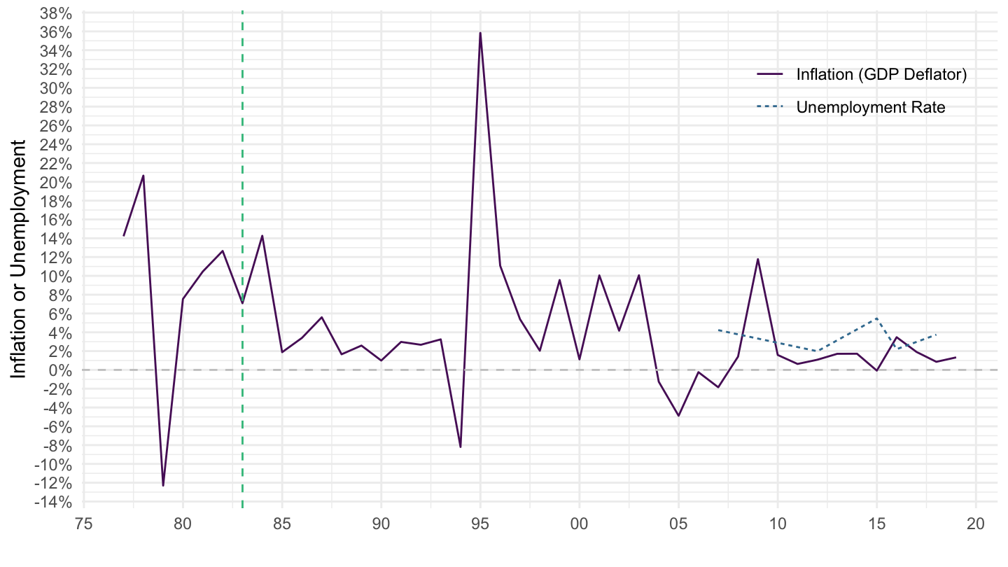
UNE_DEAP_SEX_AGE_RT_A |>
  filter(ref_area %in% c("MLI"),
         sex == "SEX_T",
         classif1 == "AGE_AGGREGATE_YGE15") |>
  mutate(date = paste0(time, "-12-31") |> as.Date()) |>
  select(date, value = obs_value) |>
  mutate(variable = "Unemployment Rate") |>
  bind_rows(NY.GDP.DEFL.KD.ZG |>
              filter(iso2c %in% c("ML")) |>
              mutate(date = paste0(year, "-12-31") |> as.Date()) |>
              select(date, value = value) |>
              mutate(variable = "Inflation (GDP Deflator)")) |>
  filter(date >= as.Date("1976-01-01")) |>
  ggplot() + geom_line() + theme_minimal() +
  aes(x = date, y = value/100, color = variable, linetype = variable) +
  xlab("") + ylab("Inflation or Unemployment") +
  scale_color_manual(values = viridis(4)[1:3]) +
  theme(legend.title = element_blank(),
        legend.position = c(0.85, 0.85)) +
  scale_x_date(breaks = seq(1900, 2100, 5) |> paste0("-01-01") |> as.Date(),
               labels = date_format("%Y")) +
  scale_y_continuous(breaks = 0.01*seq(-100, 10000, 2),
                     labels = percent_format(a = 1)) +
  geom_vline(xintercept = as.Date("1983-01-01"), linetype = "dashed", color = viridis(4)[3]) +
  geom_hline(yintercept = 0, linetype = "dashed", color = "grey")