Consumer Price Index - CPI
Data - GFD
François Geerolf
Variables
cpi_info %>%
  select(Ticker, Country) %>%
  right_join(cpi %>%
               group_by(Ticker) %>%
               summarise(Nobs = n(),
                         start = first(year(date)),
                         end = last(year(date))), by = "Ticker") %>%
  arrange(-Nobs) %>%
  mutate(Flag = gsub(" ", "-", str_to_lower(Country)),
         Flag = paste0('<img src="../../icon/flag/vsmall/', Flag, '.png" alt="Flag">')) %>%
  select(Flag, everything()) %>%
  {if (is_html_output()) datatable(., filter = 'top', rownames = F, escape = F) else .}
Individual Countries
Germany
All
cpi %>%
  filter(Ticker == "CPDEUM") %>%
  ggplot(.) +
  geom_line(aes(x = date, y = value)) +
  ylab("Price Level") + xlab("") +
  geom_rect(data = nber_recessions,
            aes(xmin = Peak, xmax = Trough, ymin = -Inf, ymax = +Inf),
            fill = 'grey', alpha = 0.5) +
  scale_y_log10(breaks =  seq(0, 1000, 20)) +
  scale_x_date(breaks = as.Date(paste0(seq(1780, 2020, 20), "-01-01")),
               labels = date_format("%Y")) +
  theme_minimal() +
  geom_vline(xintercept = as.Date("1929-10-29"), linetype = "dashed", color = "red")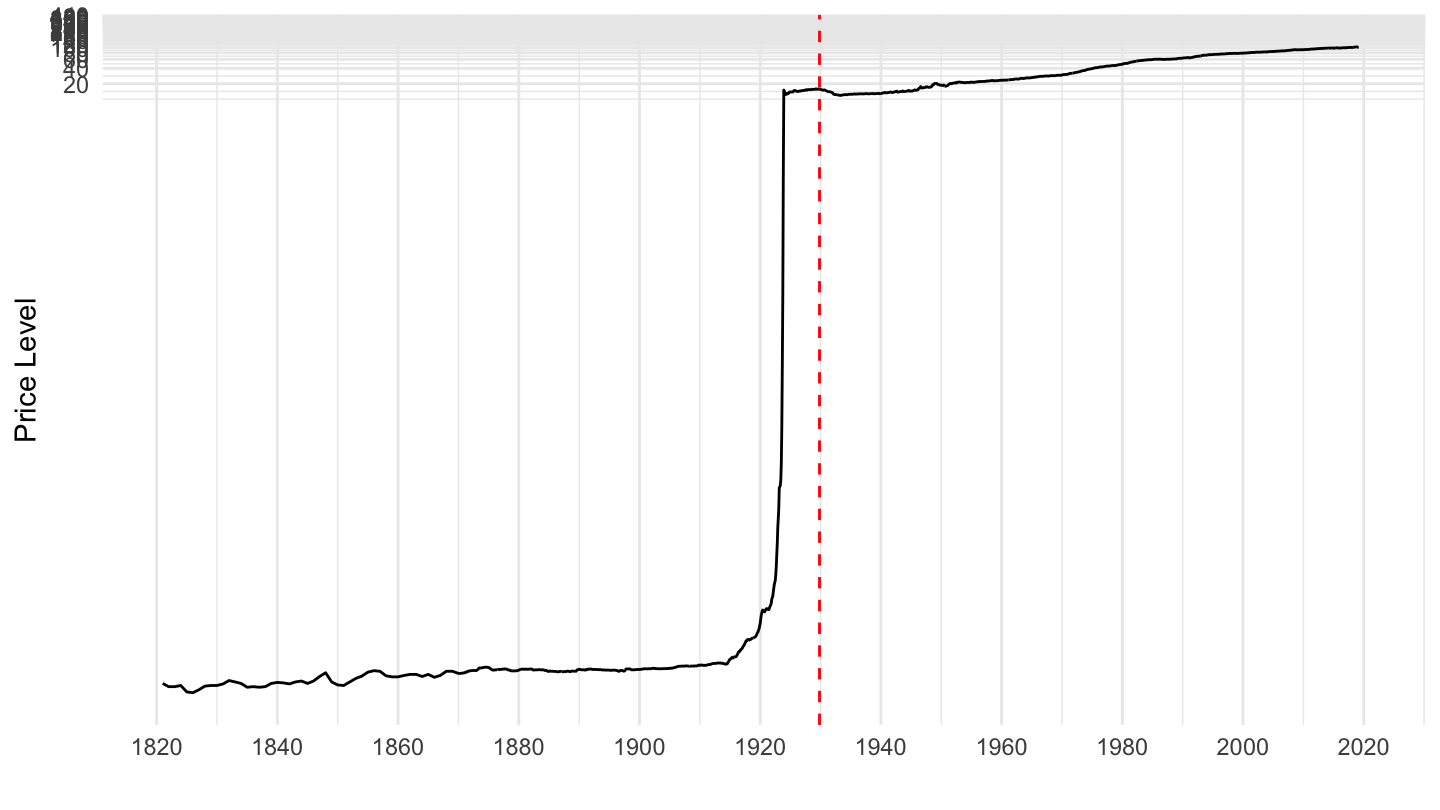
1930-
cpi %>%
  filter(Ticker == "CPDEUM",
         date >= as.Date("1930-01-01")) %>%
  ggplot(.) +
  geom_line(aes(x = date, y = value)) +
  ylab("Price Level") + xlab("") +
  scale_y_log10(breaks =  seq(0, 1000, 20)) +
  scale_x_date(breaks = as.Date(paste0(seq(1780, 2020, 20), "-01-01")),
               labels = date_format("%y")) +
  theme_minimal() +
  geom_vline(xintercept = as.Date("1929-10-29"), linetype = "dashed", color = "red")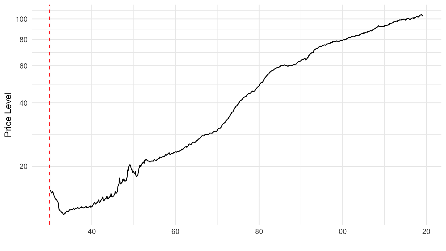
1950-
cpi %>%
  filter(Ticker == "CPDEUM",
         date >= as.Date("1950-01-01")) %>%
  ggplot(.) +
  geom_line(aes(x = date, y = value)) +
  ylab("Price Level") + xlab("") +
  scale_y_log10(breaks =  seq(0, 1000, 20)) +
  scale_x_date(breaks = as.Date(paste0(seq(1780, 2020, 20), "-01-01")),
               labels = date_format("%y")) +
  theme_minimal()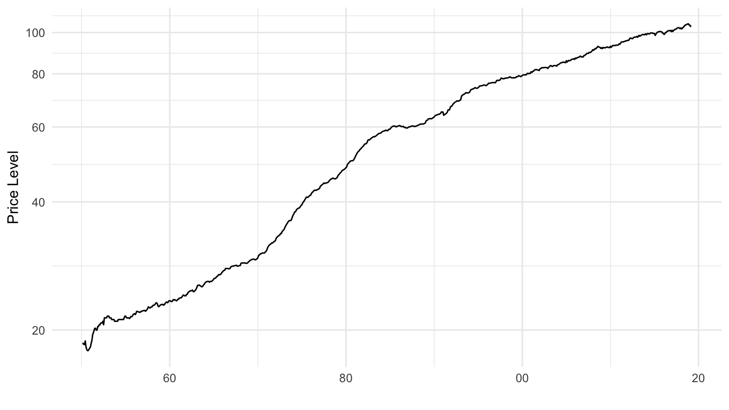
France
1950-
cpi %>%
  filter(Ticker == "CPFRAM",
         date >= as.Date("1950-01-01")) %>%
  ggplot(.) +
  geom_line(aes(x = date, y = value)) +
  ylab("Price Level") + xlab("") +
  scale_y_log10(breaks =  seq(0, 1000, 20)) +
  scale_x_date(breaks = as.Date(paste0(seq(1780, 2020, 20), "-01-01")),
               labels = date_format("%y")) +
  theme_minimal()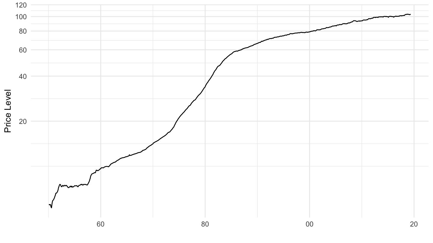
Italy
1950-
cpi %>%
  filter(Ticker == "CPITAM",
         date >= as.Date("1950-01-01")) %>%
  ggplot(.) +
  geom_line(aes(x = date, y = value)) +
  ylab("Price Level") + xlab("") +
  scale_y_log10(breaks =  seq(0, 1000, 20)) +
  scale_x_date(breaks = as.Date(paste0(seq(1780, 2020, 20), "-01-01")),
               labels = date_format("%y")) +
  theme_minimal()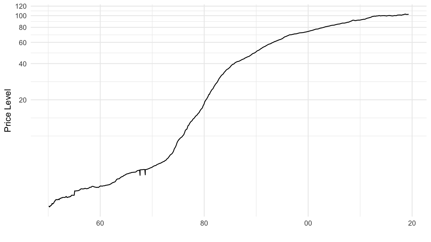
France, Italy, Germany
1950-
cpi %>%
  filter(Ticker %in% c("CPITAM", "CPFRAM", "CPDEUM"),
         date >= as.Date("1949-01-01"),
         date <= as.Date("1971-01-01")) %>%
  group_by(Ticker) %>%
  mutate(value = 100*value/value[date == as.Date("1949-01-31")]) %>%
  left_join(iso3c, by = "iso3c") %>%
  ggplot(.) + ylab("Niveau des prix (100 = 1949)") + xlab("") + theme_minimal() +
  geom_line(aes(x = date, y = value, color = Iso3c)) +
  scale_y_log10(breaks =  seq(0, 1000, 20)) +
  scale_x_date(breaks = as.Date(paste0(seq(1780, 2020, 1), "-01-01")),
               labels = date_format("%y")) +
  scale_color_manual(values = viridis(4)[1:3]) +
  theme(legend.position = c(0.2, 0.80),
        legend.title = element_blank())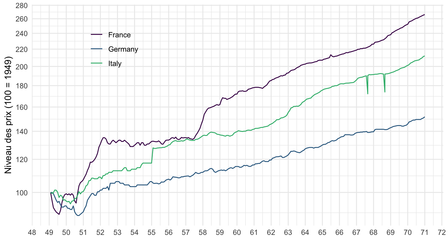
1950- (Flags)
cpi %>%
  filter(Ticker %in% c("CPFRAM", "CPITAM", "CPDEUM"),
         date >= as.Date("1949-01-01"),
         date <= as.Date("1971-01-01")) %>%
  group_by(Ticker) %>%
  mutate(value = 100*value/value[date == as.Date("1949-01-31")]) %>%
  left_join(iso3c, by = "iso3c") %>%
  ggplot(.) + ylab("Niveau des prix (100 = 1949)") + xlab("") + theme_minimal() +
  geom_line(aes(x = date, y = value, color = Iso3c)) +
  scale_y_log10(breaks =  seq(0, 1000, 20)) +
  geom_image(data = tibble(date = rep(as.Date("1971-01-01"), 3),
                           value = c(240, 140, 190),
                           image = c("~/Dropbox/bib/flags/france.png",
                                     "~/Dropbox/bib/flags/germany.png",
                                     "~/Dropbox/bib/flags/italy.png")),
             aes(x = date, y = value, image = image), asp = 1.5) +
  scale_x_date(breaks = as.Date(paste0(seq(1780, 2020, 2), "-01-01")),
               labels = date_format("%y")) +
  #geom_vline(xintercept = as.Date("1957-08-11"), color = "#0055a4", linetype = "dashed") +
  #geom_vline(xintercept = as.Date("1958-12-27"), color = "#0055a4", linetype = "dashed") +
  #geom_vline(xintercept = as.Date("1969-08-10"), color = "#0055a4", linetype = "dashed") +
  # France Blue: "#0055a4"
  # Germany Black:
  # Italian green: "#008c45"
  scale_color_manual(values = c("#0055a4", "#000000", "#008c45")) +
  theme(legend.position = "none")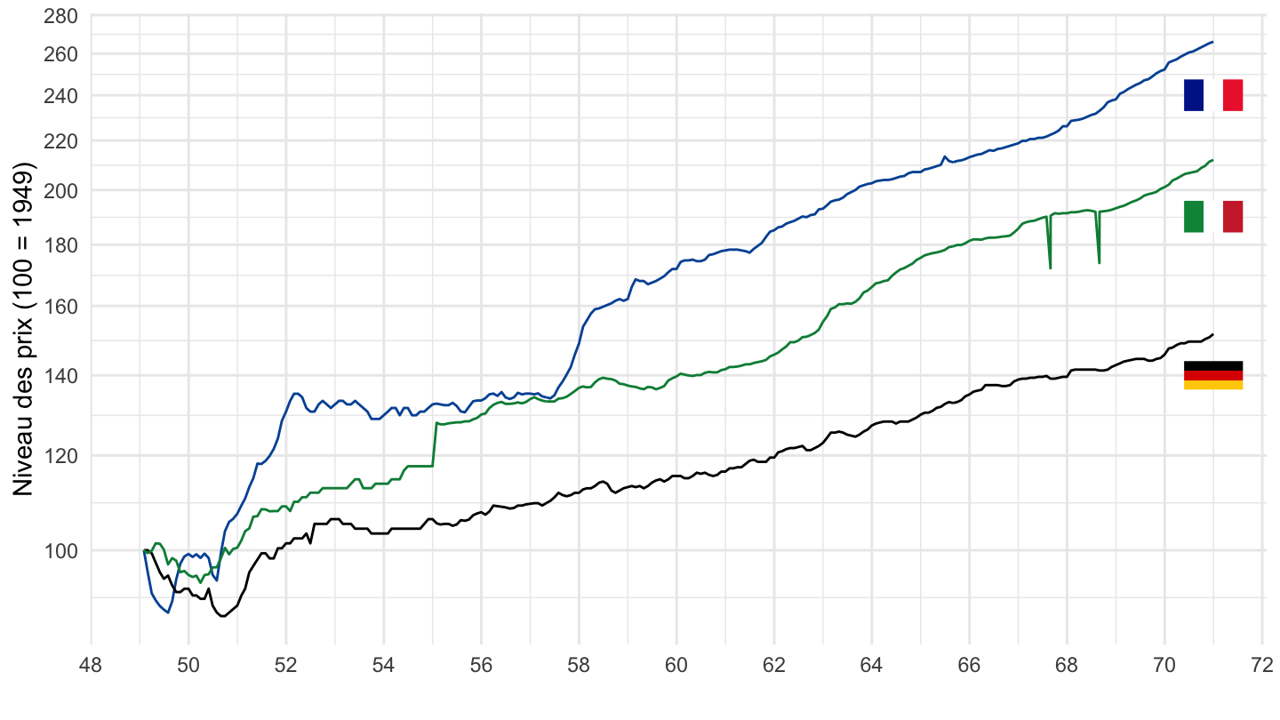
U.S.
CPI (1780-2020)
cpi %>%
  filter(Ticker == "CPUSAM") %>%
  ggplot(.) +
  geom_line(aes(x = date, y = value)) +
  ylab("Price Level") + xlab("") +
  geom_rect(data = nber_recessions,
            aes(xmin = Peak, xmax = Trough, ymin = -Inf, ymax = +Inf),
            fill = 'grey', alpha = 0.5) +
  scale_y_continuous(breaks =  seq(0, 1000, 20)) +
  scale_x_date(breaks = as.Date(paste0(seq(1780, 2020, 20), "-01-01")),
               labels = date_format("%Y")) +
  theme_minimal() +
  geom_vline(xintercept = as.Date("1929-10-29"), linetype = "dashed", color = "red")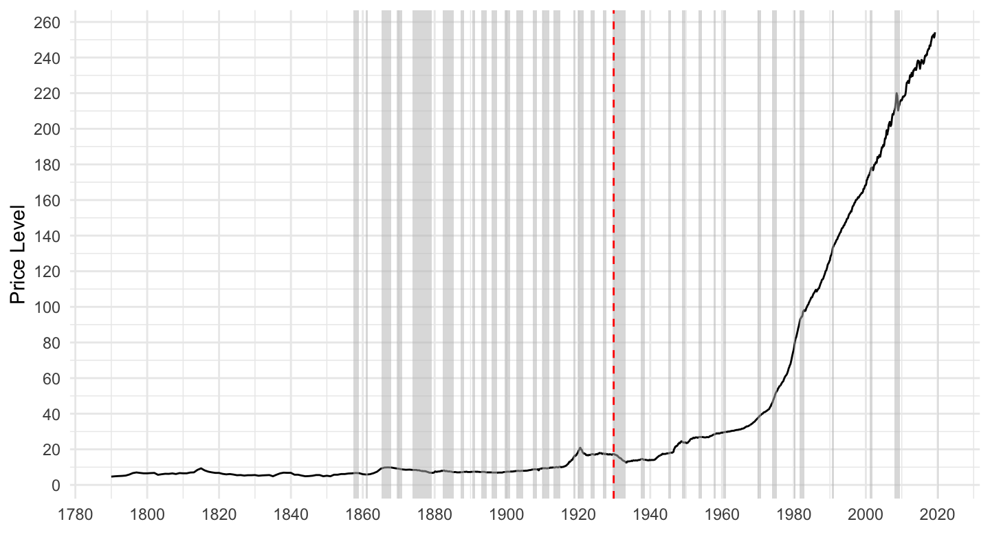
Figure 1: U.S. Price Level (1780-2020)
Log CPI (1780-2020)
cpi %>%
  filter(Ticker == "CPUSAM") %>%
  ggplot(.) +
  geom_line(aes(x = date, y = value)) +
  ylab("Price Level") + xlab("") +
  geom_rect(data = nber_recessions,
            aes(xmin = Peak, xmax = Trough, ymin = -Inf, ymax = +Inf),
            fill = 'grey', alpha = 0.5) +
  scale_y_log10(breaks =  c(25, 50, 100, 200, 300, 400)) +
  scale_x_date(breaks = as.Date(paste0(seq(1780, 2020, 20), "-01-01")),
               labels = date_format("%Y")) +
  theme_minimal() +
  geom_vline(xintercept = as.Date("1929-10-29"), linetype = "dashed", color = "red")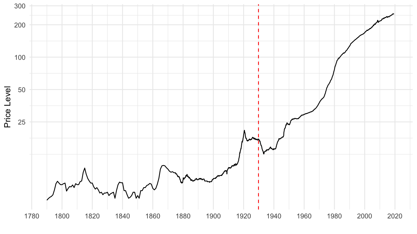
Figure 2: U.S. Price Level (1780-2020)
Argentina
1900-1960
cpi %>%
  filter(iso3c == "ARG") %>%
  filter(date >= as.Date("1900-01-01"),
         date <= as.Date("1960-01-01")) %>%
  mutate(value = 1*value/value[date == as.Date("1900-12-31")]) %>%
  ggplot(.) + theme_minimal() + ylab("Price Level") + xlab("") +
  geom_line(aes(x = date, y = value)) +
  scale_y_log10(breaks =  c(seq(0, 10, 1), seq(0, 100, 10))) +
  scale_x_date(breaks = seq(1800, 2040, 5) %>% paste0("-01-01") %>% as.Date(),
               labels = date_format("%y"))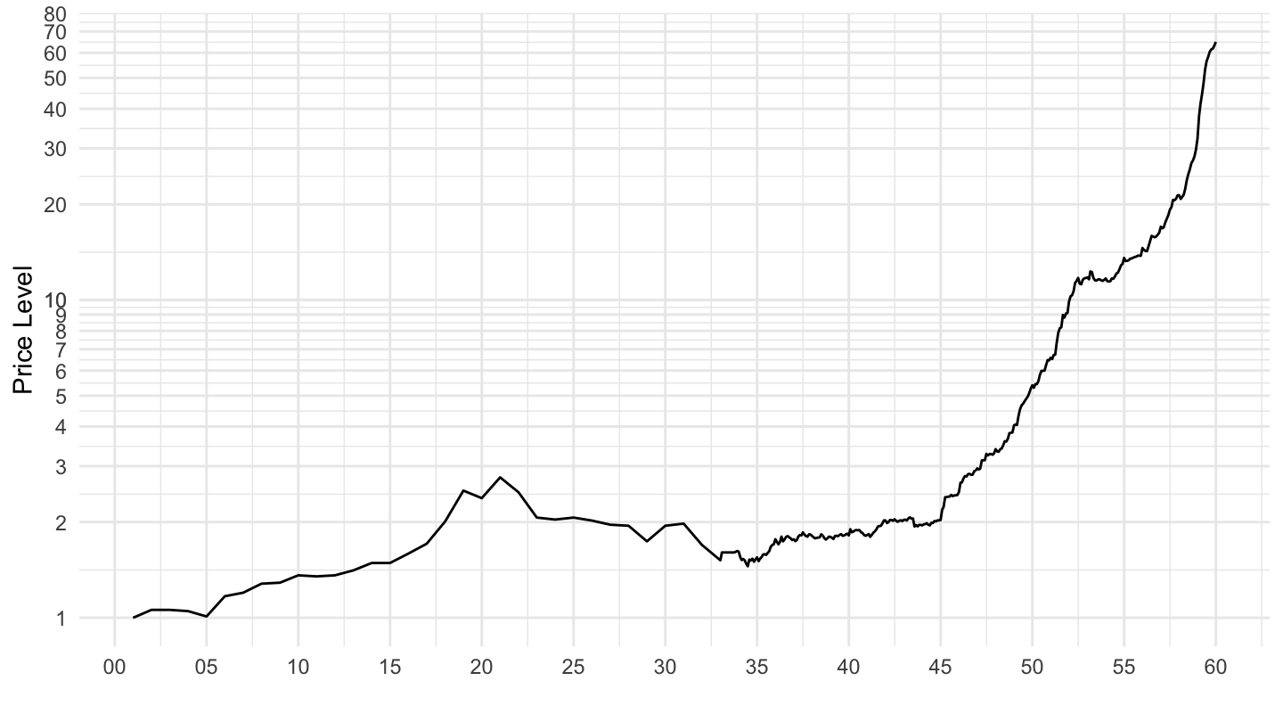
1900-1940
cpi %>%
  filter(iso3c == "ARG") %>%
  filter(date >= as.Date("1900-01-01"),
         date <= as.Date("1940-01-01")) %>%
  mutate(value = 100*value/value[date == as.Date("1900-12-31")]) %>%
  ggplot(.) + theme_minimal() + ylab("Price Level") + xlab("") +
  geom_line(aes(x = date, y = value)) +
  scale_y_log10(breaks =  c(seq(100, 200, 10), seq(200, 400, 20))) +
  scale_x_date(breaks = seq(1800, 2040, 5) %>% paste0("-01-01") %>% as.Date(),
               labels = date_format("%Y"))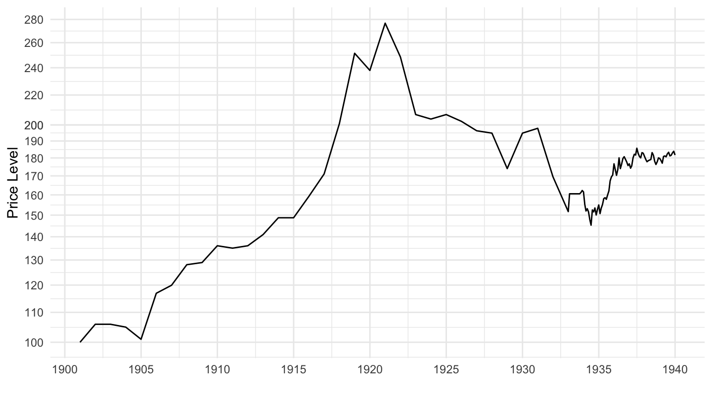
1900-1940
cpi %>%
  filter(iso3c == "ARG") %>%
  filter(date >= as.Date("1900-01-01"),
         date <= as.Date("1940-01-01")) %>%
  mutate(value = 100*value/value[date == as.Date("1900-12-31")]) %>%
  ggplot(.) + theme_minimal() + ylab("Price Level") + xlab("") +
  geom_line(aes(x = date, y = value)) +
  geom_rect(data = data_frame(start = as.Date("1921-01-01"),
                              end = as.Date("1934-04-01")),
            aes(xmin = start, xmax = end, ymin = 0, ymax = +Inf),
            fill = viridis(3)[3], alpha = 0.2) +
  scale_y_log10(breaks =  c(seq(100, 200, 10), seq(200, 400, 20))) +
  scale_x_date(breaks = seq(1800, 2040, 5) %>% paste0("-01-01") %>% as.Date(),
               labels = date_format("%Y"))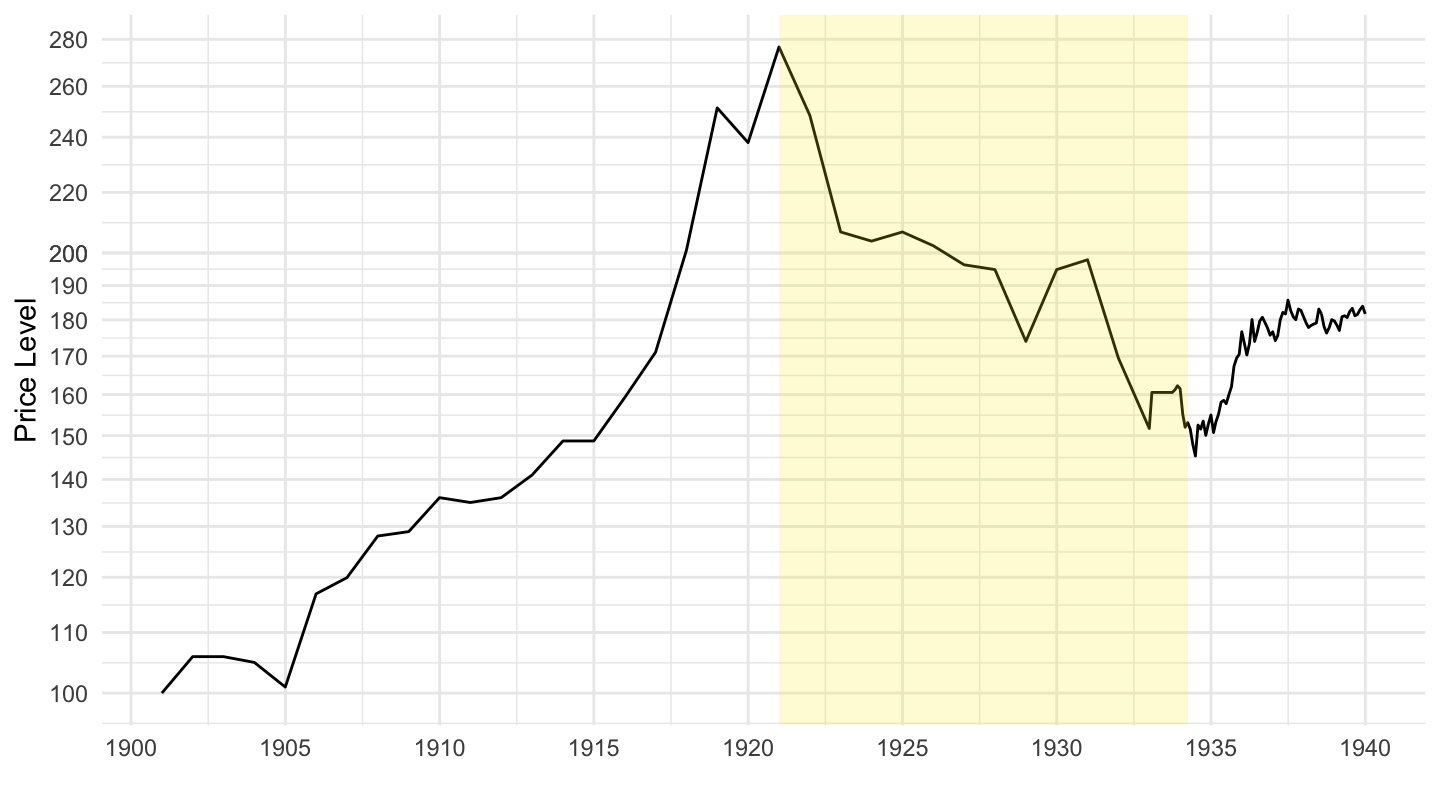
Japan
1980-1995
cpi %>%
  filter(Ticker == "CPJPNM") %>%
  filter(date >= as.Date("1980-01-01"),
         date <= as.Date("1995-01-01")) %>%
  ggplot(.) +
  geom_line(aes(x = date, y = value)) +
  ylab("Price Level") + xlab("") +
  scale_y_continuous(breaks =  seq(0, 100, 2)) +
  scale_x_date(breaks = seq(1800, 2040, 1) %>% paste0("-01-01") %>% as.Date(),
               labels = date_format("%y")) +
  theme_minimal()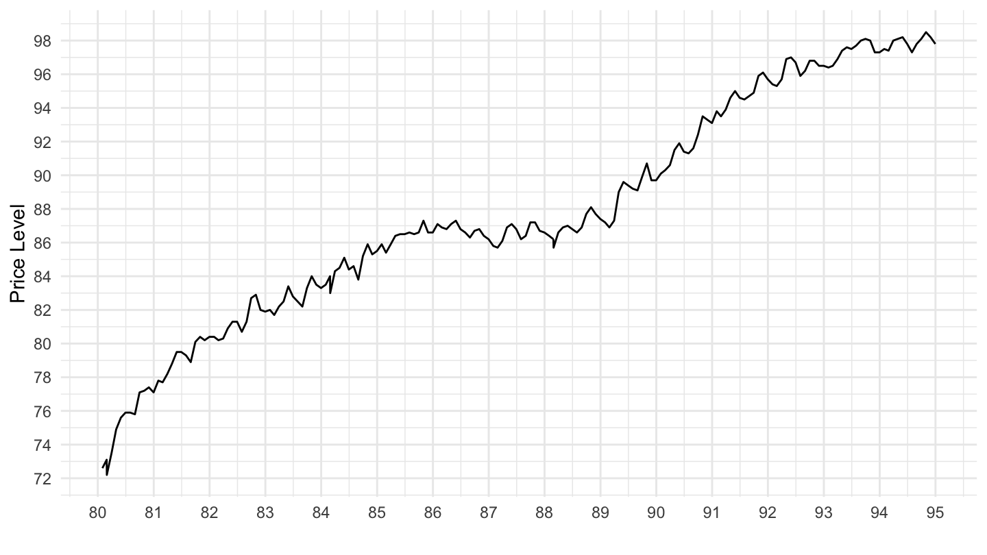
1995-2020
cpi %>%
  filter(Ticker == "CPJPNM") %>%
  filter(date >= as.Date("1995-01-01"),
         date <= as.Date("2020-01-01")) %>%
  ggplot(.) +
  geom_line(aes(x = date, y = value)) +
  ylab("Price Level") + xlab("") +
  scale_y_continuous(breaks =  seq(0, 200, 1)) +
  scale_x_date(breaks = seq(1800, 2040, 1) %>% paste0("-01-01") %>% as.Date(),
               labels = date_format("%y")) +
  theme_minimal()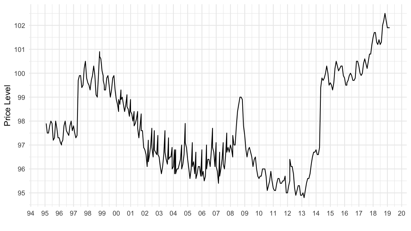
1945-2020
cpi %>%
  filter(Ticker == "CPJPNM") %>%
  filter(date >= as.Date("1945-01-01")) %>%
  ggplot(.) +
  geom_line(aes(x = date, y = value)) +
  ylab("Price Level") + xlab("") +
  scale_y_continuous(breaks =  seq(0, 100, 10)) +
  scale_x_date(breaks = seq(1800, 2040, 10) %>% paste0("-01-01") %>% as.Date(),
               labels = date_format("%y")) +
  theme_minimal() +
  geom_vline(xintercept = as.Date("1929-10-29"), linetype = "dashed", color = "red")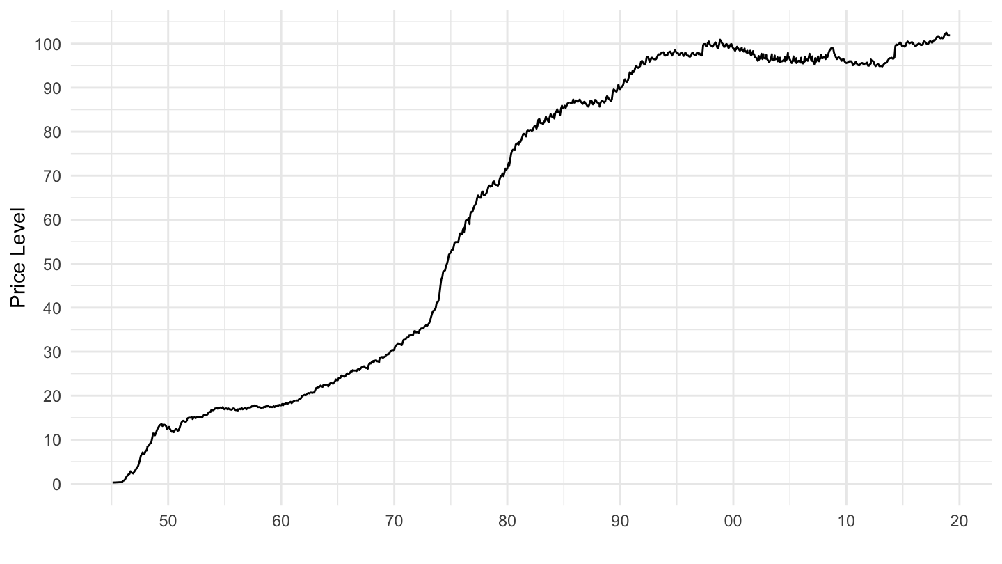
1868-2019
cpi %>%
  filter(Ticker == "CPJPNM") %>%
  filter(date <= as.Date("1945-01-01")) %>%
  ggplot(.) +
  geom_line(aes(x = date, y = value)) +
  ylab("Price Level") + xlab("") +
  scale_y_continuous(breaks =  seq(0, 0.35, 0.05),
                     limits = c(0, 0.35)) +
  scale_x_date(breaks = seq(1800, 2040, 10) %>% paste0("-01-01") %>% as.Date(),
               labels = date_format("%Y")) +
  theme_minimal() +
  geom_vline(xintercept = as.Date("1929-10-29"), linetype = "dashed", color = "red")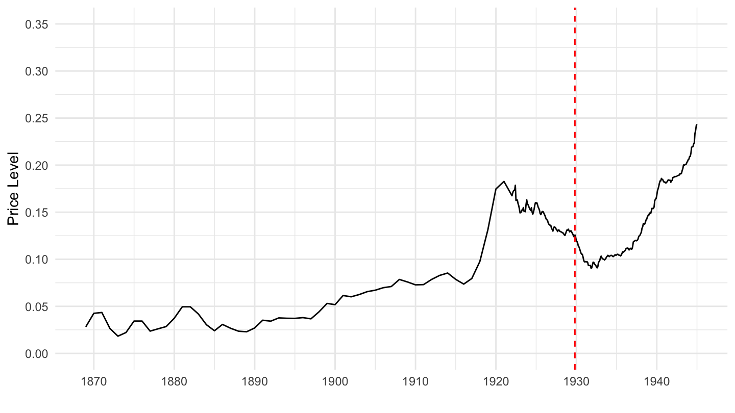
1930s Gold Standard
Eichengreen, Sachs (1985)
include_graphics2("https://fgeerolf.com/bib/EichengreenSachs1985/tab1.png")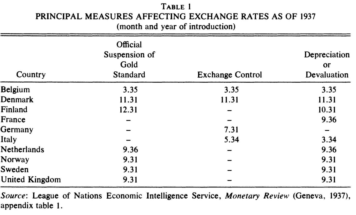
Belgium, Denmark, Finland
Without Dates
cpi %>%
  filter(iso3c %in% c("BEL", "DNK", "FIN"),
         variable == "CPM",
         date >= as.Date("1925-01-01"),
         date <= as.Date("1940-01-01")) %>%
  left_join(iso3c, by = "iso3c") %>%
  group_by(iso3c) %>%
  mutate(value = 100*value / value[date == as.Date("1925-03-31")]) %>%
  ggplot(.) + geom_line() +
  aes(x = date, y = value, color = Iso3c, linetype = Iso3c) +
  theme_minimal() + xlab("") + ylab("Price Index (Log Scale, 1925 = 100)") +
  scale_x_date(breaks = seq(1925, 2020, 1) %>% paste0("-01-01") %>% as.Date,
               labels = date_format("%y")) +
  scale_y_log10(breaks = seq(0, 200, 5),
                labels = dollar_format(accuracy = 1, prefix = "")) +
  scale_color_manual(values = viridis(4)[1:3]) +
  theme(legend.position = c(0.7, 0.90),
        legend.title = element_blank(),
        legend.direction = "horizontal")
Dates
cpi %>%
  filter(iso3c %in% c("BEL", "DNK", "FIN"),
         variable == "CPM",
         date >= as.Date("1925-01-01"),
         date <= as.Date("1940-01-01")) %>%
  left_join(iso3c, by = "iso3c") %>%
  group_by(iso3c) %>%
  mutate(value = 100*value / value[date == as.Date("1925-03-31")]) %>%
  ggplot(.) + geom_line() +
  aes(x = date, y = value, color = Iso3c, linetype = Iso3c) +
  theme_minimal() + xlab("") + ylab("Price Index (Log Scale, 1925 = 100)") +
  scale_x_date(breaks = seq(1925, 2020, 1) %>% paste0("-01-01") %>% as.Date,
               labels = date_format("%y")) +
  scale_y_log10(breaks = seq(0, 200, 5),
                labels = dollar_format(accuracy = 1, prefix = "")) +
  scale_color_manual(values = viridis(4)[1:3]) +
  theme(legend.position = c(0.7, 0.90),
        legend.title = element_blank(),
        legend.direction = "horizontal") +
  geom_vline(xintercept = as.Date("1935-03-01"), linetype = "dotted", color = viridis(4)[1]) +
  geom_vline(xintercept = as.Date("1931-11-01"), linetype = "dotted", color = viridis(4)[2]) +
  geom_vline(xintercept = as.Date("1931-12-01"), linetype = "dotted", color = viridis(4)[3])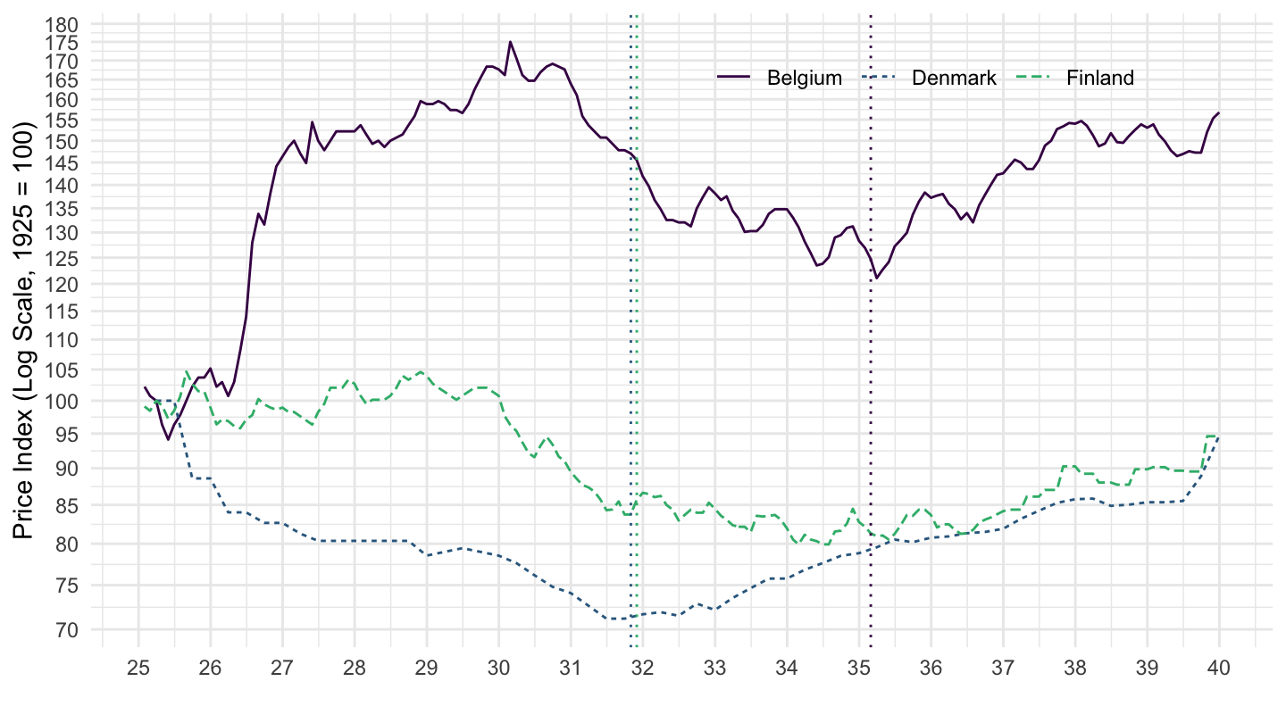
France - CPI (1900-1940)
cpi %>%
  filter(variable == "CPM",
         iso3c == "FRA") %>%
  ggplot(.) +
  geom_line(aes(x = date, y = value)) +
  ylab("Price Level") + xlab("") +
  scale_y_continuous(breaks =  seq(0, 0.35, 0.05),
                     limits = c(0, 0.35)) +
  scale_x_date(breaks = seq(1900, 1940, 5) %>% paste0("-01-01") %>% as.Date(),
               labels = date_format("%Y"),
               limits = c(1900, 1940) %>% paste0("-01-01") %>% as.Date) +
  theme_minimal() +
  geom_vline(xintercept = as.Date("1929-10-29"), linetype = "dashed", color = "red")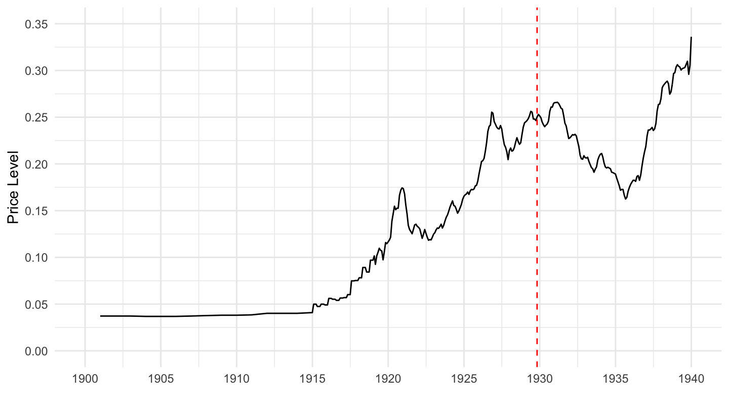
Figure 3: France Price Level (1900-1940)
France, Germany, Italy
Without Dates
cpi %>%
  filter(iso3c %in% c("FRA", "DEU", "ITA"),
         variable == "CPM",
         date >= as.Date("1925-01-01"),
         date <= as.Date("1940-01-01")) %>%
  left_join(iso3c, by = "iso3c") %>%
  group_by(iso3c) %>%
  mutate(value = 100*value / value[date == as.Date("1925-03-31")]) %>%
  ggplot(.) + geom_line() +
  aes(x = date, y = value, color = Iso3c, linetype = Iso3c) +
  theme_minimal() + xlab("") + ylab("Price Index (Log Scale, 1925 = 100)") +
  scale_x_date(breaks = seq(1925, 2020, 1) %>% paste0("-01-01") %>% as.Date,
               labels = date_format("%y")) +
  scale_y_log10(breaks = seq(0, 200, 5),
                labels = dollar_format(accuracy = 1, prefix = "")) +
  scale_color_manual(values = viridis(4)[1:3]) +
  theme(legend.position = c(0.7, 0.90),
        legend.title = element_blank(),
        legend.direction = "horizontal")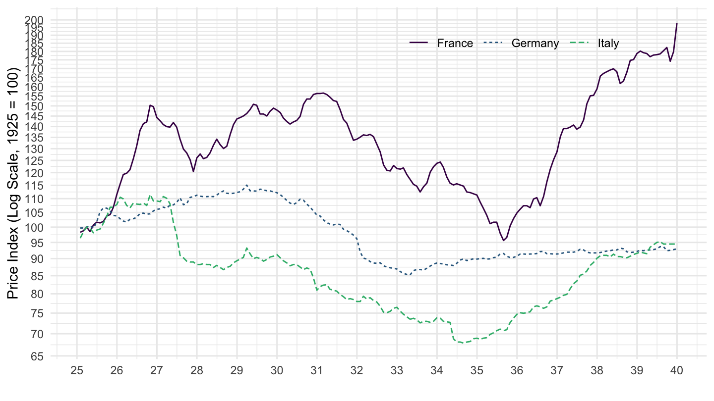
Dates
cpi %>%
  filter(iso3c %in% c("FRA", "DEU", "ITA"),
         variable == "CPM",
         date >= as.Date("1925-01-01"),
         date <= as.Date("1940-01-01")) %>%
  left_join(iso3c, by = "iso3c") %>%
  group_by(iso3c) %>%
  mutate(value = 100*value / value[date == as.Date("1925-03-31")]) %>%
  ggplot(.) + geom_line() +
  aes(x = date, y = value, color = Iso3c, linetype = Iso3c) +
  theme_minimal() + xlab("") + ylab("Price Index (Log Scale, 1925 = 100)") +
  scale_x_date(breaks = seq(1925, 2020, 1) %>% paste0("-01-01") %>% as.Date,
               labels = date_format("%y")) +
  scale_y_log10(breaks = seq(0, 200, 5),
                labels = dollar_format(accuracy = 1, prefix = "")) +
  scale_color_manual(values = viridis(4)[1:3]) +
  theme(legend.position = c(0.7, 0.90),
        legend.title = element_blank(),
        legend.direction = "horizontal") +
  geom_vline(xintercept = as.Date("1936-09-01"), linetype = "dotted", color = viridis(4)[1]) +
  geom_vline(xintercept = as.Date("1931-07-01"), linetype = "dotted", color = viridis(4)[2]) +
  geom_vline(xintercept = as.Date("1934-05-01"), linetype = "dotted", color = viridis(4)[3])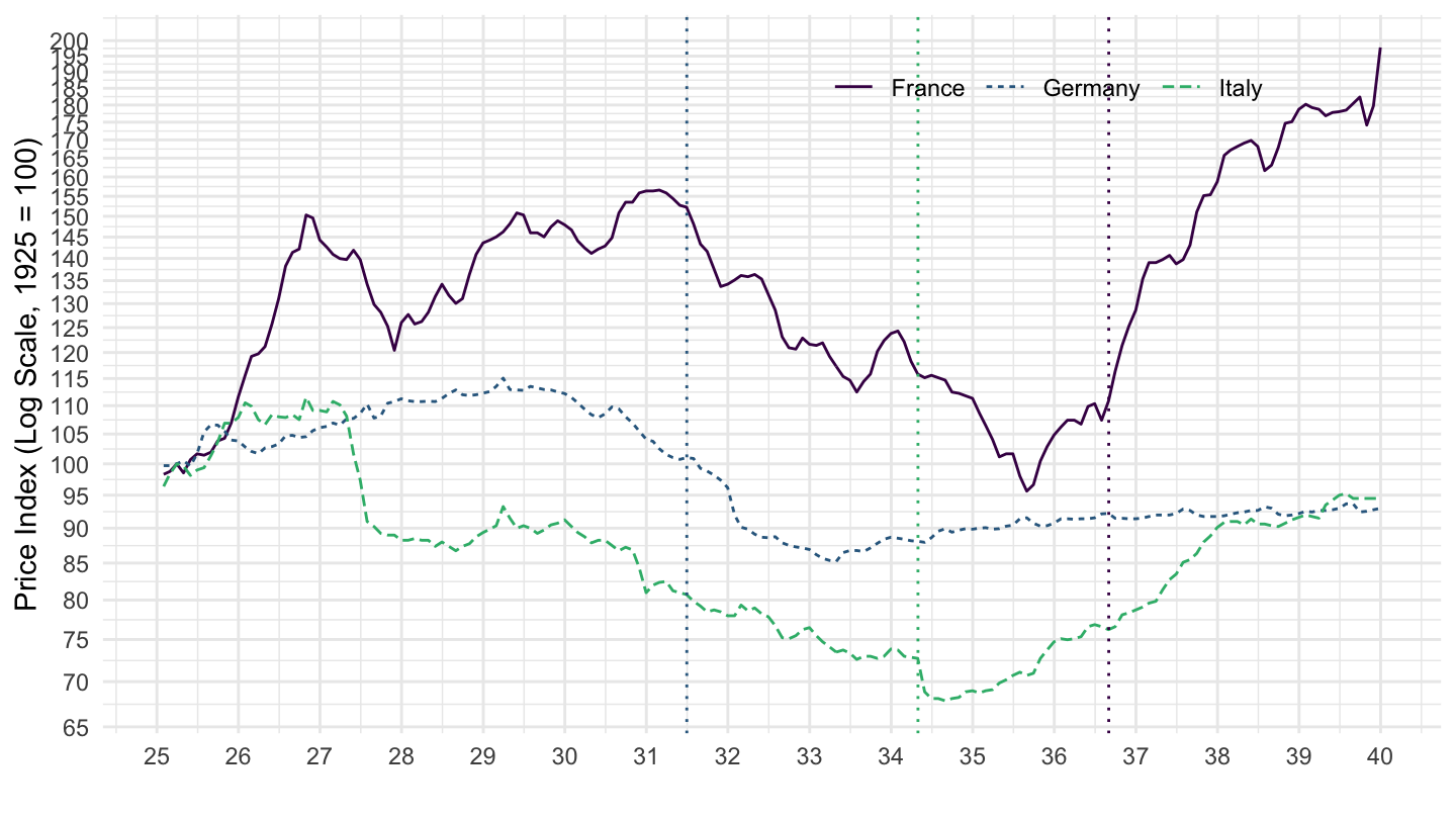
Netherlands, Norway, Sweden
Without Dates
cpi %>%
  filter(iso3c %in% c("NLD", "NOR", "SWE"),
         variable == "CPM",
         date >= as.Date("1925-01-01"),
         date <= as.Date("1940-01-01")) %>%
  left_join(iso3c, by = "iso3c") %>%
  group_by(iso3c) %>%
  mutate(value = 100*value / value[date == as.Date("1925-03-31")]) %>%
  ggplot(.) + geom_line() +
  aes(x = date, y = value, color = Iso3c, linetype = Iso3c) +
  theme_minimal() + xlab("") + ylab("Price Index (Log Scale, 1925 = 100)") +
  scale_x_date(breaks = seq(1925, 2020, 1) %>% paste0("-01-01") %>% as.Date,
               labels = date_format("%y")) +
  scale_y_log10(breaks = seq(0, 200, 5),
                labels = dollar_format(accuracy = 1, prefix = "")) +
  scale_color_manual(values = viridis(4)[1:3]) +
  theme(legend.position = c(0.65, 0.90),
        legend.title = element_blank(),
        legend.direction = "horizontal")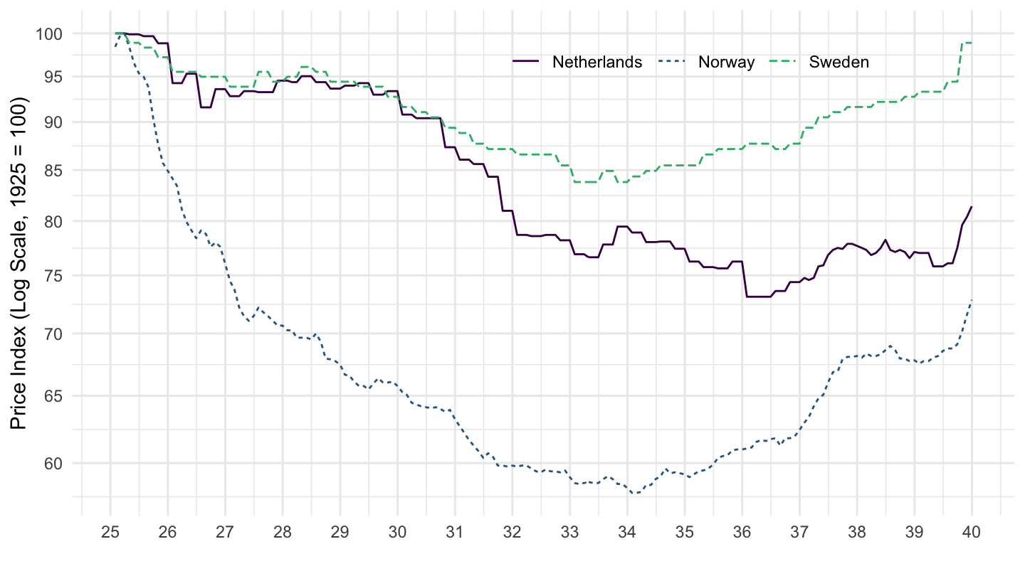
Dates
cpi %>%
  filter(iso3c %in% c("NLD", "NOR", "SWE"),
         variable == "CPM",
         date >= as.Date("1925-01-01"),
         date <= as.Date("1940-01-01")) %>%
  left_join(iso3c, by = "iso3c") %>%
  group_by(iso3c) %>%
  mutate(value = 100*value / value[date == as.Date("1925-03-31")]) %>%
  ggplot(.) + geom_line() +
  aes(x = date, y = value, color = Iso3c, linetype = Iso3c) +
  theme_minimal() + xlab("") + ylab("Price Index (Log Scale, 1925 = 100)") +
  scale_x_date(breaks = seq(1925, 2020, 1) %>% paste0("-01-01") %>% as.Date,
               labels = date_format("%y")) +
  scale_y_log10(breaks = seq(0, 200, 5),
                labels = dollar_format(accuracy = 1, prefix = "")) +
  scale_color_manual(values = viridis(4)[1:3]) +
  theme(legend.position = c(0.65, 0.90),
        legend.title = element_blank(),
        legend.direction = "horizontal") +
  geom_vline(xintercept = as.Date("1936-09-01"), linetype = "dotted", color = viridis(4)[1]) +
  geom_vline(xintercept = as.Date("1931-09-01"), linetype = "dotted", color = viridis(4)[2]) +
  geom_vline(xintercept = as.Date("1931-09-01"), linetype = "dotted", color = viridis(4)[3])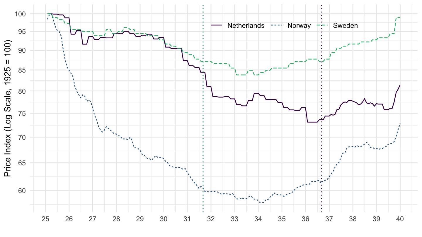
United States, United Kingdom
Without Dates
cpi %>%
  filter(iso3c %in% c("USA", "GBR"),
         variable == "CPM",
         date >= as.Date("1925-01-01"),
         date <= as.Date("1940-01-01")) %>%
  left_join(iso3c, by = "iso3c") %>%
  group_by(iso3c) %>%
  mutate(value = 100*value / value[date == as.Date("1925-01-31")]) %>%
  ggplot(.) + geom_line() +
  aes(x = date, y = value, color = Iso3c, linetype = Iso3c) +
  theme_minimal() + xlab("") + ylab("Price Index (Log Scale, 1925 = 100)") +
  scale_x_date(breaks = seq(1925, 2020, 1) %>% paste0("-01-01") %>% as.Date,
               labels = date_format("%y")) +
  scale_y_log10(breaks = seq(0, 200, 5),
                labels = dollar_format(accuracy = 1, prefix = "")) +
  scale_color_manual(values = viridis(5)[1:4]) +
  theme(legend.position = c(0.7, 0.90),
        legend.title = element_blank(),
        legend.direction = "horizontal")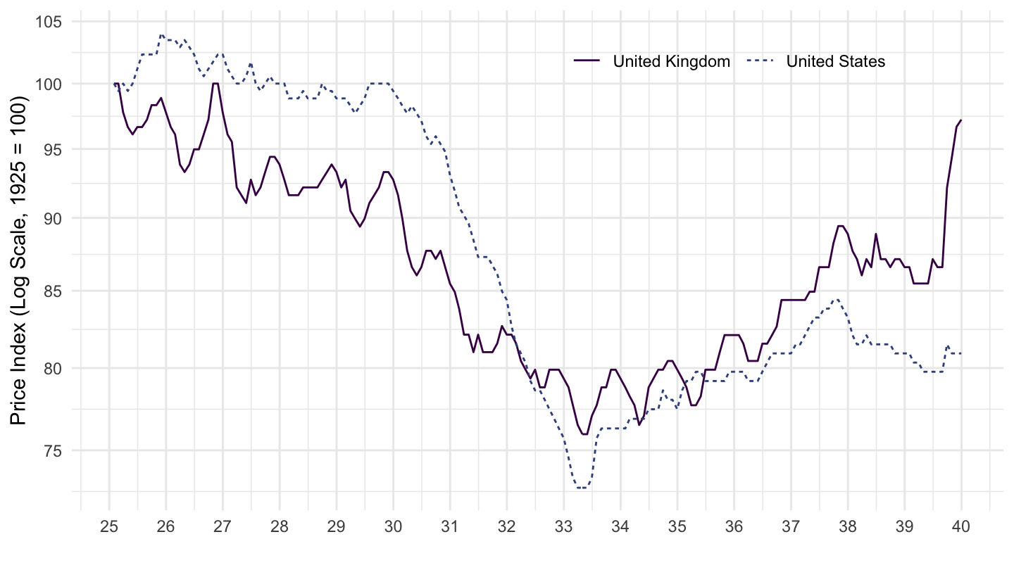
Dates
cpi %>%
  filter(iso3c %in% c("USA", "GBR"),
         variable == "CPM",
         date >= as.Date("1925-01-01"),
         date <= as.Date("1940-01-01")) %>%
  left_join(iso3c, by = "iso3c") %>%
  group_by(iso3c) %>%
  mutate(value = 100*value / value[date == as.Date("1925-01-31")]) %>%
  ggplot(.) + geom_line() +
  aes(x = date, y = value, color = Iso3c, linetype = Iso3c) +
  theme_minimal() + xlab("") + ylab("Price Index (Log Scale, 1925 = 100)") +
  scale_x_date(breaks = seq(1925, 2020, 1) %>% paste0("-01-01") %>% as.Date,
               labels = date_format("%y")) +
  scale_y_log10(breaks = seq(0, 200, 5),
                labels = dollar_format(accuracy = 1, prefix = "")) +
  scale_color_manual(values = viridis(5)[1:4]) +
  theme(legend.position = c(0.7, 0.90),
        legend.title = element_blank(),
        legend.direction = "horizontal") +
  geom_vline(xintercept = as.Date("1931-09-01"), linetype = "dotted", color = viridis(4)[1]) +
  geom_vline(xintercept = as.Date("1933-03-01"), linetype = "dotted", color = viridis(4)[2])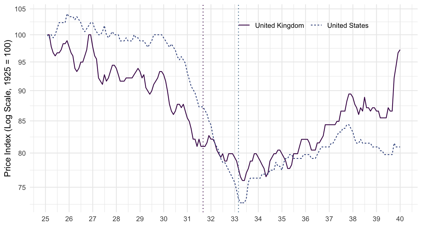
Norway, United Kingdom, Italy
cpi %>%
  filter(iso3c %in% c("NOR", "GBR", "ITA"),
         variable == "CPM",
         date >= as.Date("1925-01-01"),
         date <= as.Date("1940-01-01")) %>%
  left_join(iso3c, by = "iso3c") %>%
  group_by(iso3c) %>%
  mutate(value = 1*value / value[date == as.Date("1925-01-31")]) %>%
  ggplot(.) + geom_line() +
  aes(x = date, y = value, color = Iso3c, linetype = Iso3c) +
  theme_minimal() + xlab("") + ylab("Price Index (Log Scale, 1925 = 1)") +
  scale_x_date(breaks = seq(1925, 2020, 1) %>% paste0("-01-01") %>% as.Date,
               labels = date_format("%y")) +
  scale_y_log10(breaks = seq(0.1, 3, 0.1),
                labels = dollar_format(accuracy = .1, prefix = "")) +
  scale_color_manual(values = viridis(4)[1:3]) +
  theme(legend.position = c(0.5, 0.90),
        legend.title = element_blank(),
        legend.direction = "horizontal")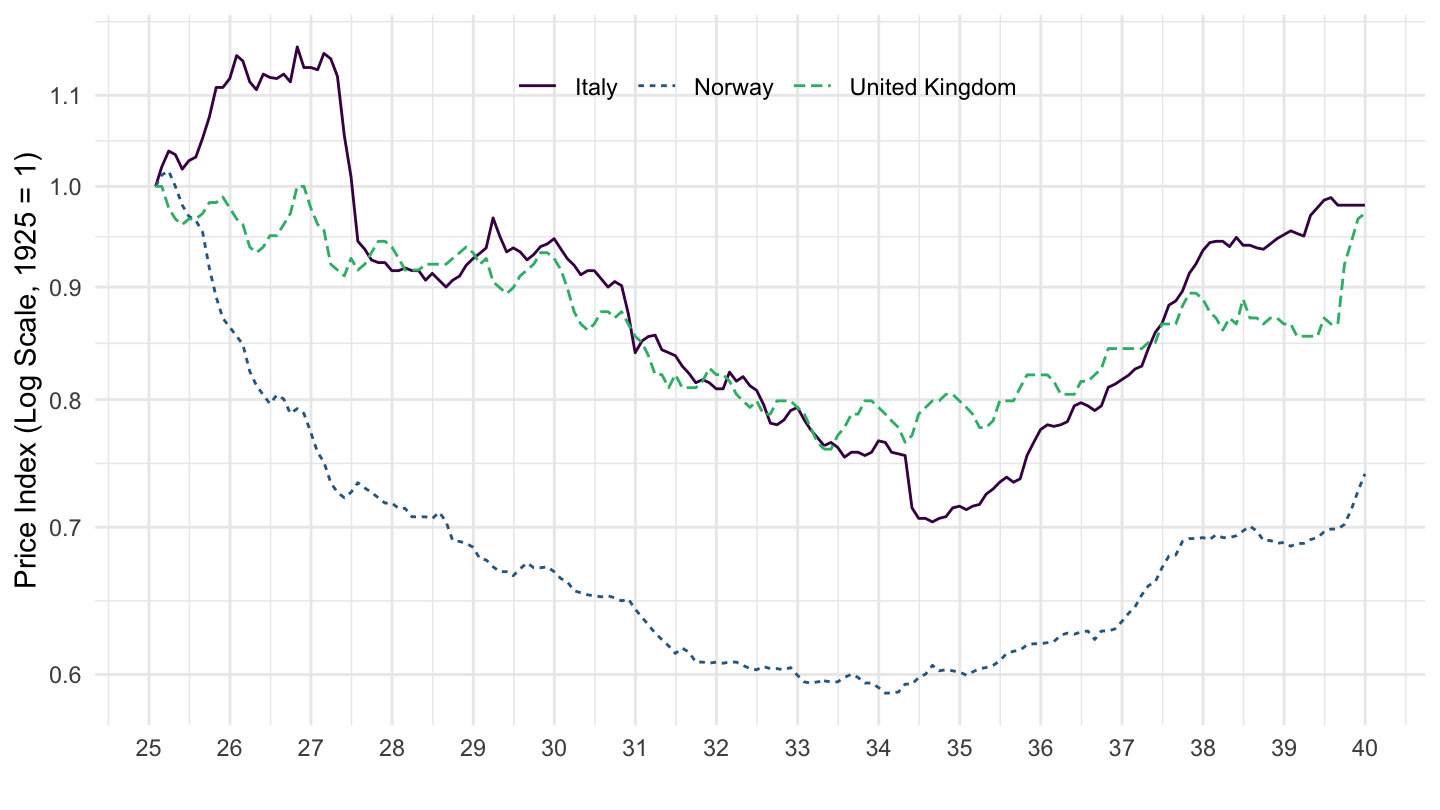
France, United Kingdom, Italy
cpi %>%
  filter(iso3c %in% c("FRA", "GBR", "ITA"),
         variable == "CPM",
         date >= as.Date("1925-01-01"),
         date <= as.Date("1940-01-01")) %>%
  left_join(iso3c, by = "iso3c") %>%
  group_by(iso3c) %>%
  mutate(value = 1*value / value[date == as.Date("1925-01-31")]) %>%
  ggplot(.) + geom_line() +
  aes(x = date, y = value, color = Iso3c, linetype = Iso3c) +
  theme_minimal() + xlab("") + ylab("Price Index (Log Scale, 1925 = 1)") +
  scale_x_date(breaks = seq(1925, 2020, 1) %>% paste0("-01-01") %>% as.Date,
               labels = date_format("%y")) +
  scale_y_log10(breaks = seq(0.1, 3, 0.1),
                labels = dollar_format(accuracy = .1, prefix = "")) +
  scale_color_manual(values = viridis(4)[1:3]) +
  theme(legend.position = c(0.3, 0.90),
        legend.title = element_blank(),
        legend.direction = "horizontal")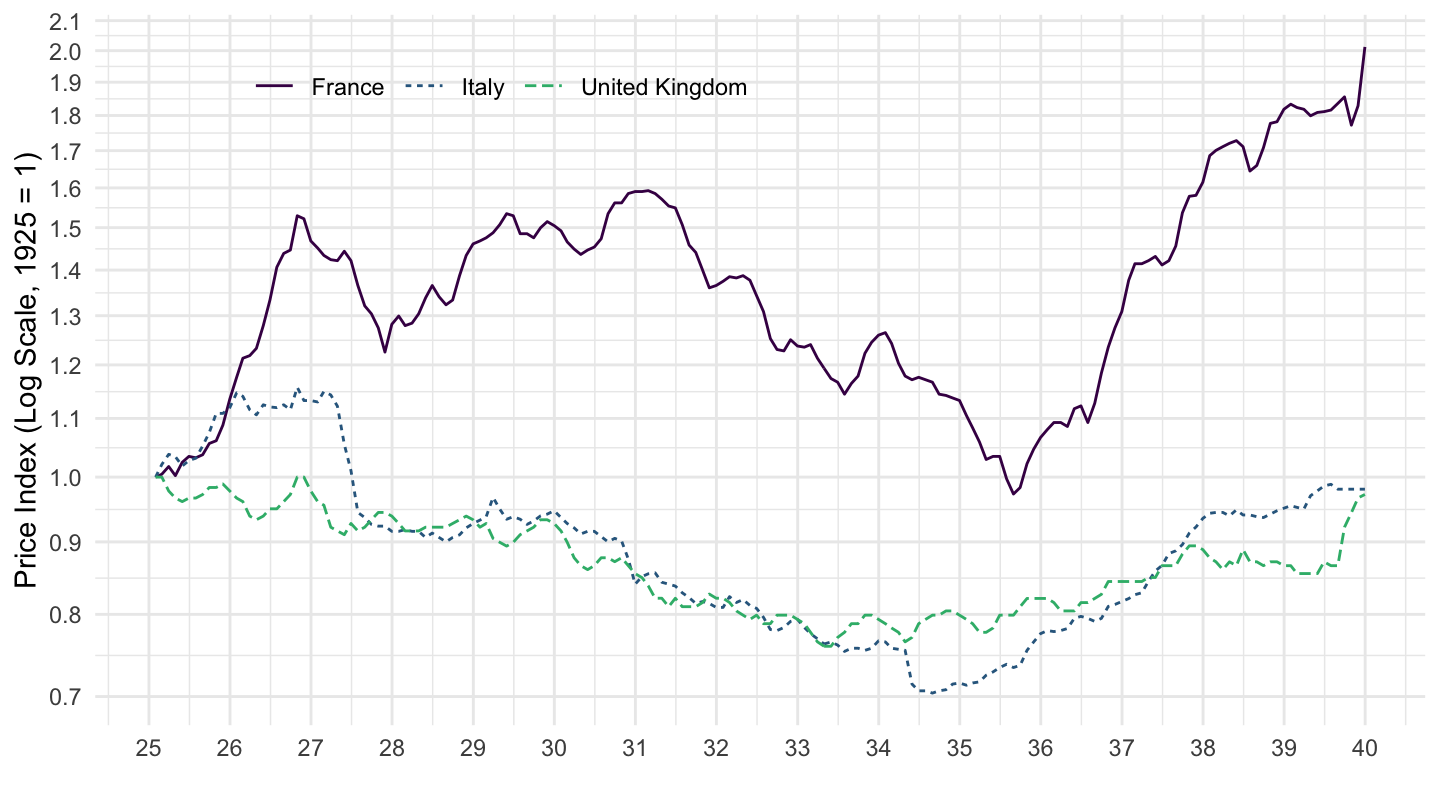
Germany, GBR, USA, FRA
cpi %>%
  filter(iso3c %in% c("DEU", "GBR", "USA", "FRA"),
         variable == "CPM",
         date >= as.Date("1925-01-01"),
         date <= as.Date("1940-01-01")) %>%
  left_join(iso3c, by = "iso3c") %>%
  group_by(iso3c) %>%
  mutate(value = 1*value / value[date == as.Date("1925-01-31")]) %>%
  ggplot(.) + geom_line() +
  aes(x = date, y = value, color = Iso3c, linetype = Iso3c) +
  theme_minimal() + xlab("") + ylab("Price Index (Log Scale, 1925 = 1)") +
  scale_x_date(breaks = seq(1925, 2020, 1) %>% paste0("-01-01") %>% as.Date,
               labels = date_format("%y")) +
  scale_y_log10(breaks = seq(0.1, 3, 0.1),
                labels = dollar_format(accuracy = .1, prefix = "")) +
  scale_color_manual(values = viridis(5)[1:4]) +
  theme(legend.position = c(0.4, 0.90),
        legend.title = element_blank(),
        legend.direction = "horizontal")
ITA, ESP, USA, FRA
cpi %>%
  filter(iso3c %in% c("ITA", "ESP", ""),
         variable == "CPM",
         date >= as.Date("1925-01-01"),
         date <= as.Date("1940-01-01")) %>%
  left_join(iso3c, by = "iso3c") %>%
  group_by(iso3c) %>%
  mutate(value = 1*value / value[date == as.Date("1925-01-31")]) %>%
  ggplot(.) + geom_line() +
  aes(x = date, y = value, color = Iso3c, linetype = Iso3c) +
  theme_minimal() + xlab("") + ylab("Price Index (Log Scale, 1925 = 1)") +
  scale_x_date(breaks = seq(1925, 2020, 1) %>% paste0("-01-01") %>% as.Date,
               labels = date_format("%y")) +
  scale_y_log10(breaks = seq(0.1, 3, 0.1),
                labels = dollar_format(accuracy = .1, prefix = "")) +
  scale_color_manual(values = viridis(5)[1:4]) +
  theme(legend.position = c(0.4, 0.90),
        legend.title = element_blank(),
        legend.direction = "horizontal")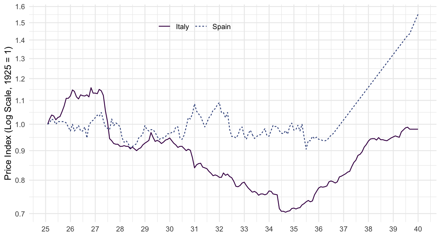
Number of observations
cpi %>%
  filter(variable == "CPM",
         date >= as.Date("1925-01-01"),
         date <= as.Date("1940-01-01")) %>%
  left_join(iso3c, by = "iso3c") %>%
  group_by(iso3c, Iso3c) %>%
  summarise(Nobs = n()) %>%
  arrange(-Nobs) %>%
  {if (is_html_output()) datatable(., filter = 'top', rownames = F) else .}
1925-1970
Deflations
cpi %>%
  filter(iso3c %in% c("DEU", "GBR", "USA"),
         variable == "CPM",
         date >= as.Date("1925-01-01"),
         date <= as.Date("1970-01-01")) %>%
  left_join(iso3c, by = "iso3c") %>%
  group_by(iso3c) %>%
  mutate(value = 1*value / value[date == as.Date("1925-01-31")]) %>%
  ggplot(.) + geom_line(aes(x = date, y = value, color = Iso3c)) +
  theme_minimal() + xlab("") + ylab("Price Index (Log Scale, 1925 = 1)") +
  scale_x_date(breaks = seq(1925, 2020, 5) %>% paste0("-01-01") %>% as.Date,
               labels = date_format("%y")) +
  scale_y_log10(breaks = seq(0.1, 3, 0.1),
                labels = dollar_format(accuracy = .1, prefix = "")) +
  scale_color_manual(values = c("#000000", "#CF142B", "#3C3B6E")) +
  geom_image(data = . %>%
               filter(date == as.Date("1940-12-31")) %>%
               mutate(image = paste0("../../icon/flag/", str_to_lower(gsub(" ", "-", Iso3c)), ".png")),
             aes(x = date, y = value, image = image), asp = 1.5) +
  theme(legend.position = c(0.2, 0.80),
        legend.title = element_blank())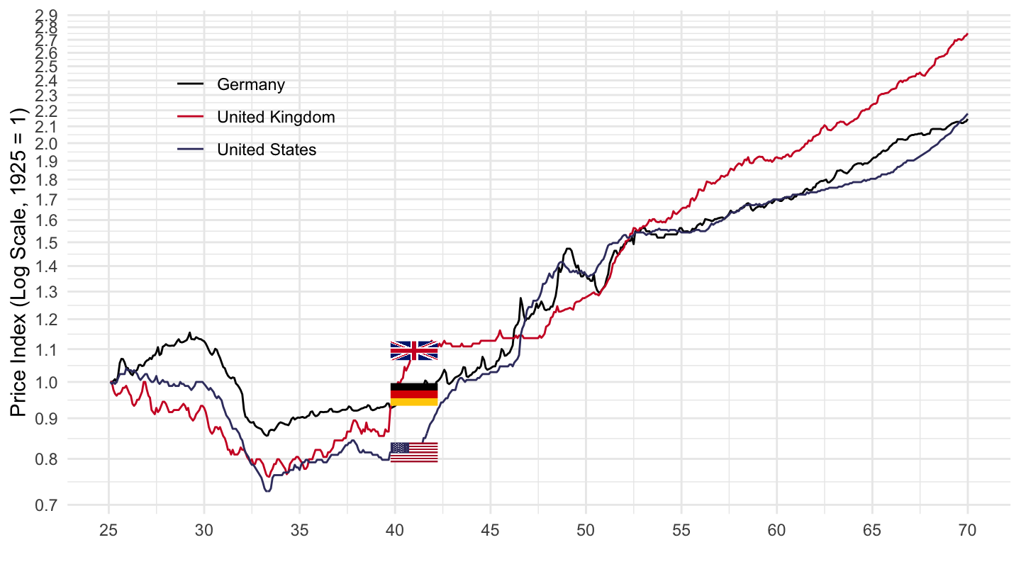
DEU, FRA, GBR, USA
cpi %>%
  filter(iso3c %in% c("DEU", "FRA", "GBR", "USA"),
         variable == "CPM",
         date >= as.Date("1925-01-01"),
         date <= as.Date("1970-01-01")) %>%
  left_join(iso3c, by = "iso3c") %>%
  group_by(iso3c) %>%
  mutate(value = 1*value / value[date == as.Date("1925-01-31")]) %>%
  ggplot(.) + geom_line() +
  aes(x = date, y = value, color = Iso3c, linetype = Iso3c) +
  theme_minimal() + xlab("") + ylab("Price Index (Log Scale, 1925 = 1)") +
  scale_x_date(breaks = seq(1925, 2020, 5) %>% paste0("-01-01") %>% as.Date,
               labels = date_format("%y")) +
  scale_y_log10(breaks = c(seq(0.1, 1, 0.1), seq(1, 10, 1), seq(10, 100, 10)),
                     labels = dollar_format(accuracy = 1, prefix = "")) +
  scale_color_manual(values = viridis(5)[1:4]) +
  theme(legend.position = c(0.2, 0.80),
        legend.title = element_blank())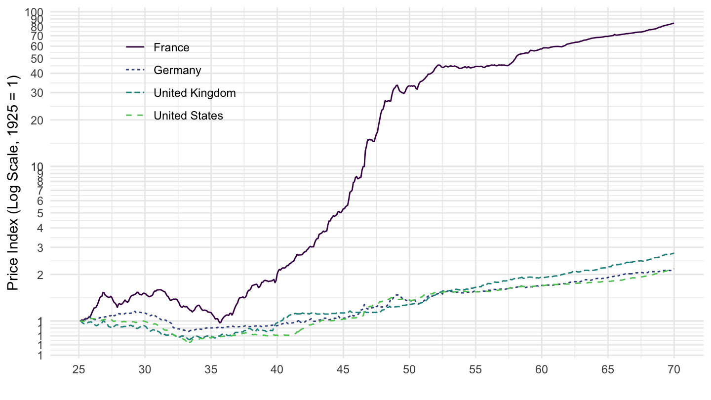
DEU, FRA, ITA, JPN, GBR
cpi %>%
  filter(iso3c %in% c("USA", "FRA", "ITA", "JPN", "GBR"),
         variable == "CPM",
         date >= as.Date("1925-01-01"),
         date <= as.Date("1970-01-01")) %>%
  left_join(iso3c, by = "iso3c") %>%
  group_by(iso3c) %>%
  mutate(value = 1*value / value[date == as.Date("1925-01-31")]) %>%
  ggplot(.) + geom_line(aes(x = date, y = value, color = Iso3c, linetype = Iso3c)) +
  theme_minimal() + xlab("") + ylab("Price Index (Log Scale, 1925 = 1)") +
  scale_x_date(breaks = seq(1925, 2020, 5) %>% paste0("-01-01") %>% as.Date,
               labels = date_format("%y")) +
  geom_image(data = . %>%
               filter(date == as.Date("1969-12-31")) %>%
               mutate(image = paste0("../../icon/flag/", str_to_lower(gsub(" ", "-", Iso3c)), ".png")),
             aes(x = date, y = value, image = image), asp = 1.5) +
  scale_y_log10(breaks = c(1, c(1, 2, 3, 5, 7, 10), 10*c(1, 2, 3, 5, 7, 10), 100*c(1, 2, 3, 5, 7, 10)),
                     labels = dollar_format(accuracy = 1, prefix = "")) +
  scale_color_manual(values = c("#000000", "#009246", "#BC002D", "#6E82B5", "#B22234")) +
  scale_linetype_manual(values = c("solid", "solid","longdash","solid",  "solid")) +
  theme(legend.position = "none")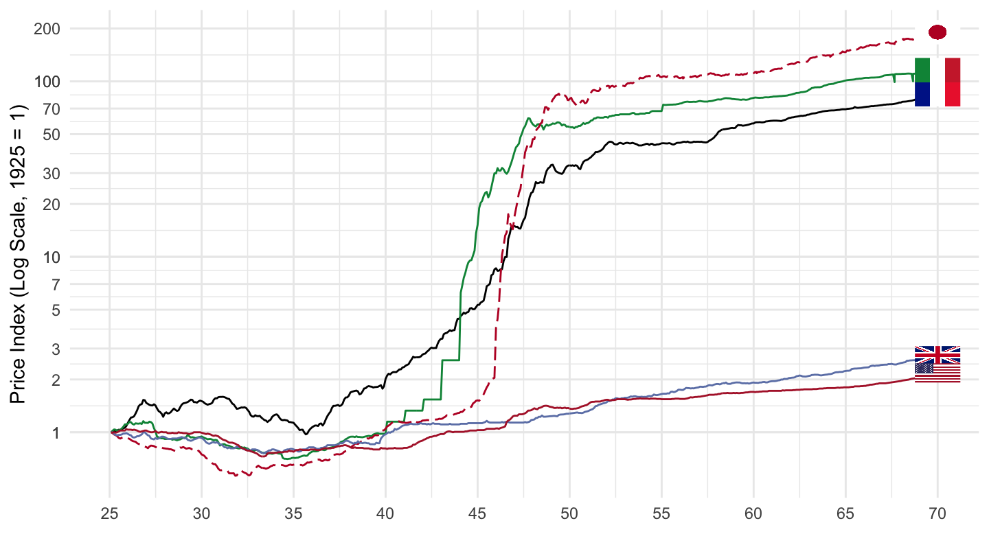
CHE, ESP, ITA, JPN
cpi %>%
  filter(iso3c %in% c("CHE", "ESP", "ITA", "JPN"),
         variable == "CPM",
         date >= as.Date("1925-01-01"),
         date <= as.Date("1970-01-01")) %>%
  left_join(iso3c, by = "iso3c") %>%
  group_by(iso3c) %>%
  mutate(value = 1*value / value[date == as.Date("1925-01-31")]) %>%
  ggplot(.) + geom_line() +
  aes(x = date, y = value, color = Iso3c, linetype = Iso3c) +
  theme_minimal() + xlab("") + ylab("Price Index (1928-06 = 1)") +
  scale_x_date(breaks = seq(1925, 2020, 5) %>% paste0("-01-01") %>% as.Date,
               labels = date_format("%y")) +
  scale_y_log10(breaks = c(1, 2, 3, 4, 5, 10, 20, 30, 40, 50, 100),
                     labels = dollar_format(accuracy = 1, prefix = "")) +
  scale_color_manual(values = viridis(5)[1:4]) +
  theme(legend.position = c(0.2, 0.80),
        legend.title = element_blank())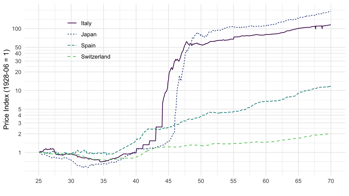
1945-1970
DEU, GBR, USA
cpi %>%
  filter(iso3c %in% c("DEU", "GBR", "USA"),
         variable == "CPM",
         date >= as.Date("1945-01-01"),
         date <= as.Date("1973-01-01")) %>%
  left_join(iso3c, by = "iso3c") %>%
  group_by(iso3c) %>%
  mutate(value = 1*value / value[date == as.Date("1945-01-31")]) %>%
  ggplot(.) + geom_line() +
  aes(x = date, y = value, color = Iso3c, linetype = Iso3c) +
  theme_minimal() + xlab("") + ylab("Price Index (Log Scale, 1945 = 1)") +
  scale_x_date(breaks = seq(1925, 2020, 5) %>% paste0("-01-01") %>% as.Date,
               labels = date_format("%y")) +
  scale_y_log10(breaks = seq(0.1, 3, 0.1),
                     labels = dollar_format(accuracy = .1, prefix = "")) +
  scale_color_manual(values = viridis(5)[1:4]) +
  theme(legend.position = c(0.2, 0.80),
        legend.title = element_blank())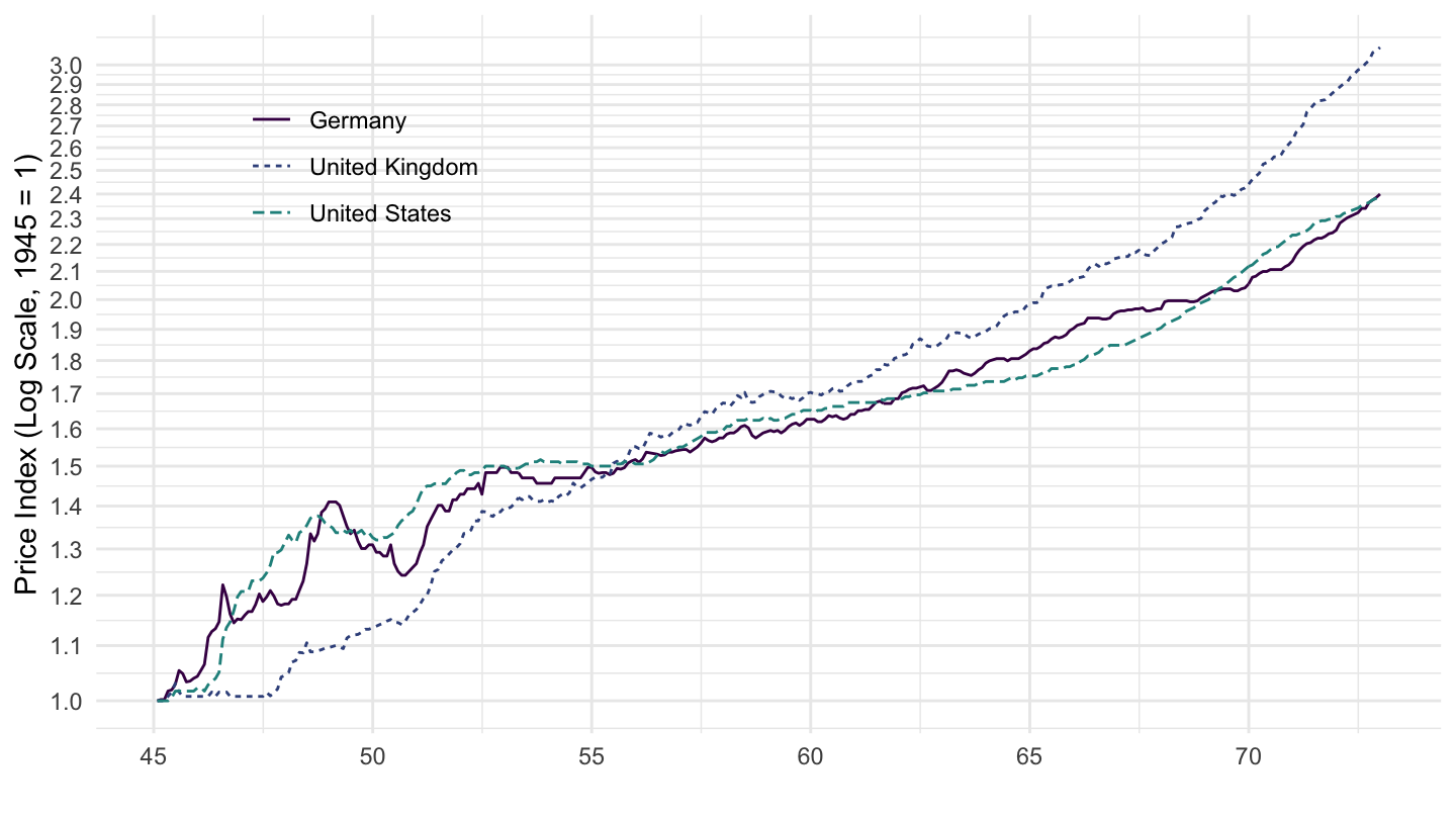
DEU, FRA, GBR, USA
cpi %>%
  filter(iso3c %in% c("DEU", "FRA", "GBR", "USA"),
         variable == "CPM",
         date >= as.Date("1945-01-01"),
         date <= as.Date("1973-01-01")) %>%
  left_join(iso3c, by = "iso3c") %>%
  group_by(iso3c) %>%
  mutate(value = 1*value / value[date == as.Date("1945-01-31")]) %>%
  ggplot(.) + geom_line() +
  aes(x = date, y = value, color = Iso3c, linetype = Iso3c) +
  theme_minimal() + xlab("") + ylab("Price Index (Log Scale, 1945 = 1)") +
  scale_x_date(breaks = seq(1925, 2020, 5) %>% paste0("-01-01") %>% as.Date,
               labels = date_format("%y")) +
  scale_y_log10(breaks = c(seq(0.1, 1, 0.1), seq(1, 10, 1), seq(10, 100, 10)),
                     labels = dollar_format(accuracy = .1, prefix = "")) +
  scale_color_manual(values = viridis(5)[1:4]) +
  theme(legend.position = c(0.15, 0.85),
        legend.title = element_blank())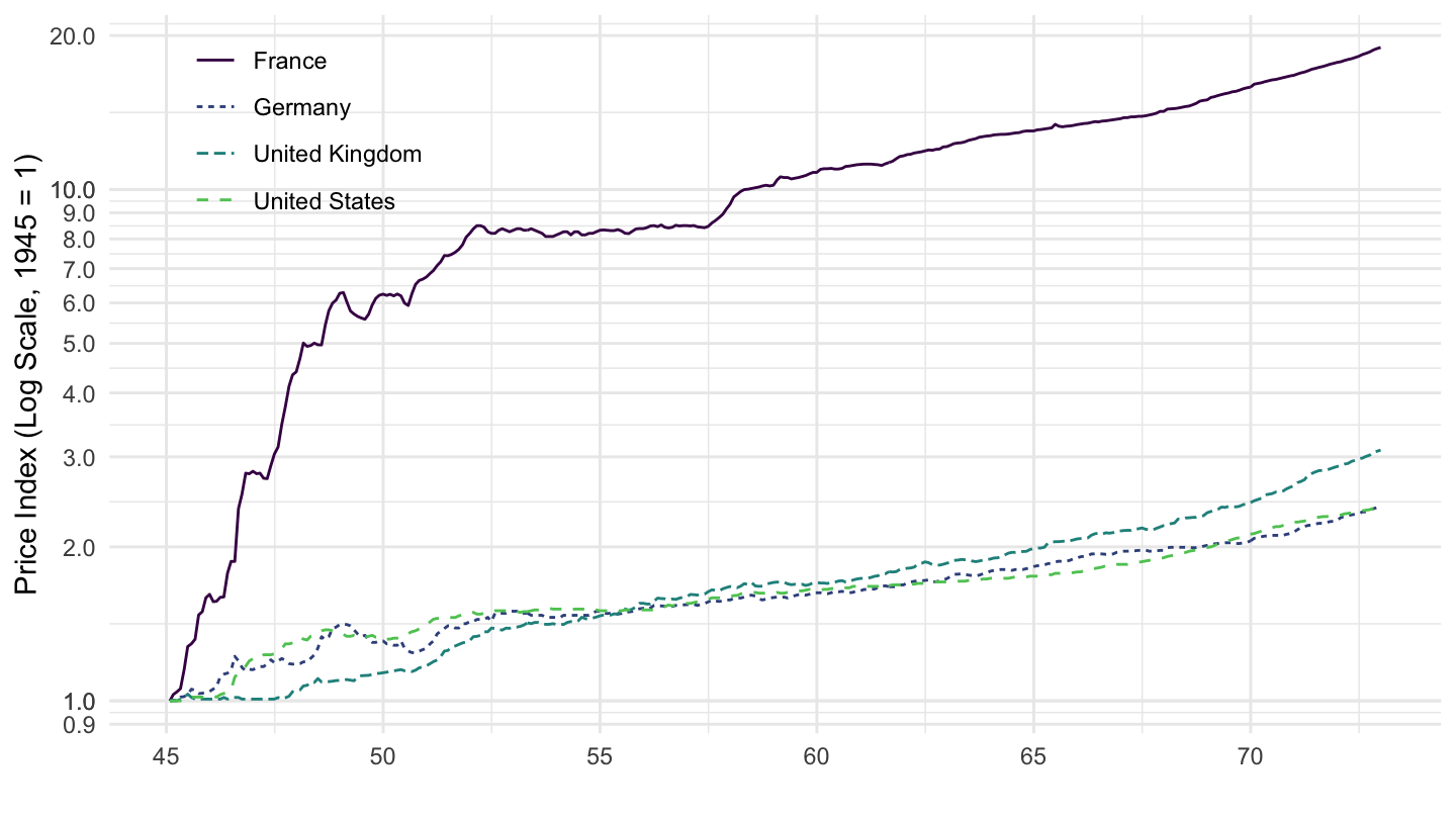
CHE, ESP, ITA, JPN
cpi %>%
  filter(iso3c %in% c("CHE", "ESP", "ITA", "JPN"),
         variable == "CPM",
         date >= as.Date("1945-01-01"),
         date <= as.Date("1973-01-01")) %>%
  left_join(iso3c, by = "iso3c") %>%
  group_by(iso3c) %>%
  mutate(value = 1*value / value[date == as.Date("1945-01-31")]) %>%
  ggplot(.) + geom_line() +
  aes(x = date, y = value, color = Iso3c, linetype = Iso3c) +
  theme_minimal() + xlab("") + ylab("Price Index (1928-06 = 1)") +
  scale_x_date(breaks = seq(1925, 2020, 5) %>% paste0("-01-01") %>% as.Date,
               labels = date_format("%y")) +
  scale_y_log10(breaks = c(1, 2, 3, 4, 5, 10, 20, 30, 40, 50, 100),
                     labels = dollar_format(accuracy = 1, prefix = "")) +
  scale_color_manual(values = viridis(5)[1:4]) +
  theme(legend.position = c(0.4, 0.6),
        legend.title = element_blank())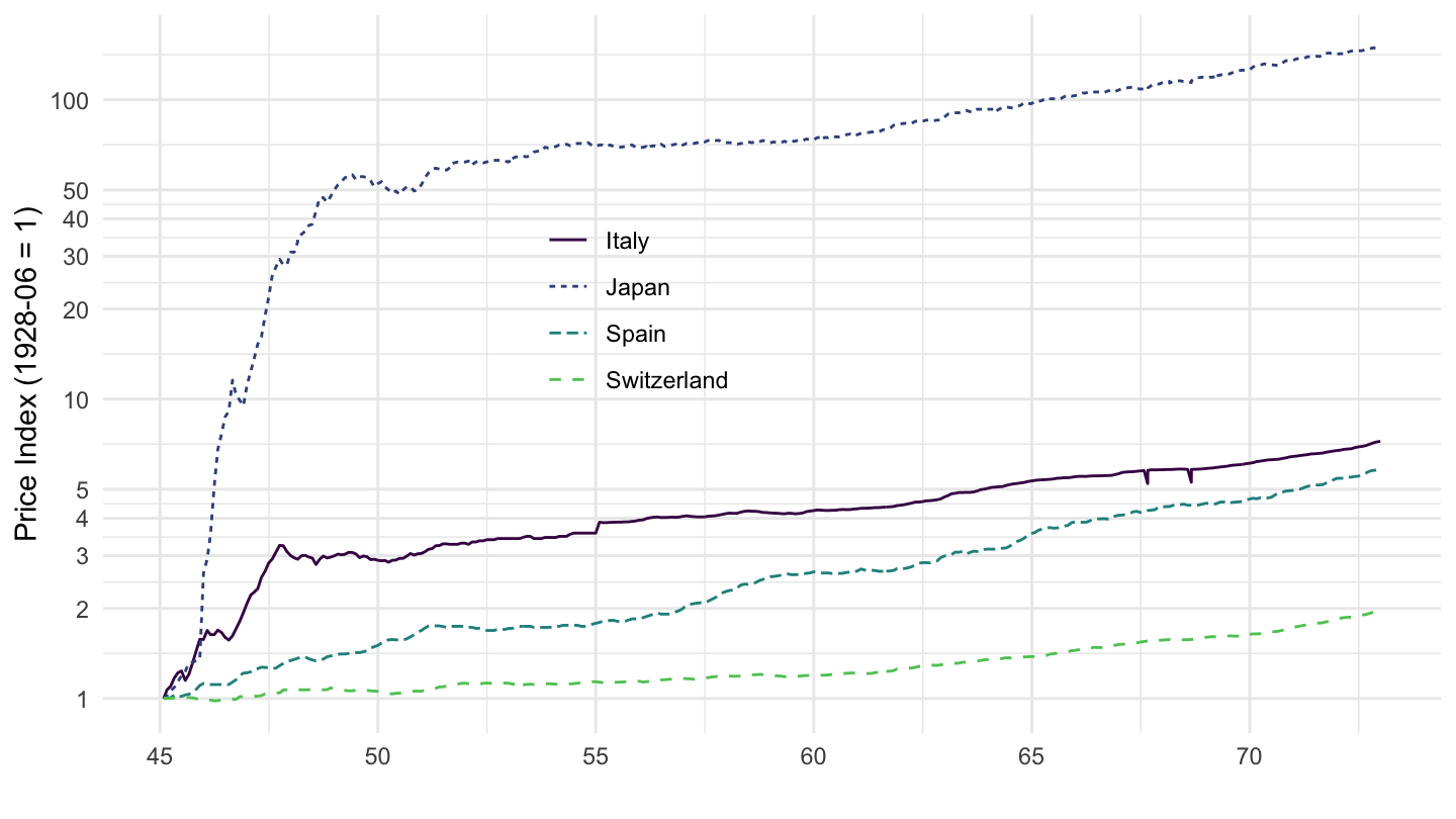
1800-1930
DEU, GBR, USA
cpi %>%
  filter(iso3c %in% c("DEU", "GBR", "USA"),
         variable == "CPM",
         date >= as.Date("1800-01-01"),
         date <= as.Date("1930-01-01")) %>%
  left_join(iso3c, by = "iso3c") %>%
  group_by(iso3c) %>%
  mutate(value = 1*value / value[date == as.Date("1820-12-31")]) %>%
  ggplot(.) + geom_line() +
  aes(x = date, y = value, color = Iso3c, linetype = Iso3c) +
  theme_minimal() + xlab("") + ylab("Price Index (Log Scale, 1945 = 1)") +
  scale_x_date(breaks = seq(1800, 2020, 20) %>% paste0("-01-01") %>% as.Date,
               labels = date_format("%Y")) +
  scale_y_log10(breaks = 10^seq(0, 20, 1),
                labels = dollar_format(accuracy = 1, prefix = "")) +
  scale_color_manual(values = viridis(5)[1:4]) +
  theme(legend.position = c(0.2, 0.80),
        legend.title = element_blank())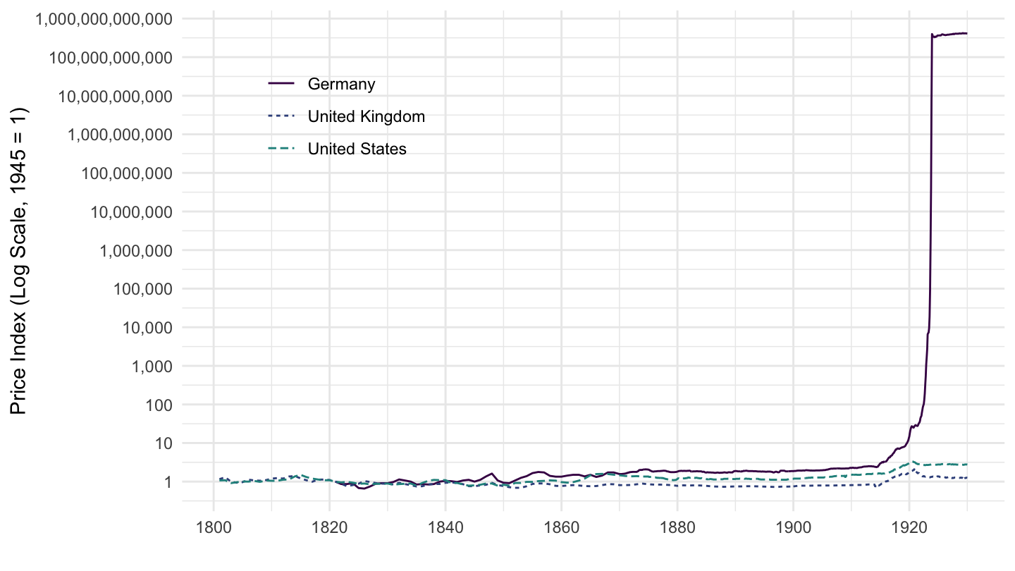
FRA, GBR, USA
cpi %>%
  filter(iso3c %in% c("FRA", "GBR", "USA"),
         variable == "CPM",
         date >= as.Date("1800-01-01"),
         date <= as.Date("1930-01-01")) %>%
  left_join(iso3c, by = "iso3c") %>%
  group_by(iso3c) %>%
  mutate(value = 1*value / value[date == as.Date("1840-12-31")]) %>%
  ggplot(.) + geom_line() +
  aes(x = date, y = value, color = Iso3c, linetype = Iso3c) +
  theme_minimal() + xlab("") + ylab("Price Index (Log Scale, 1925 = 1)") +
  scale_x_date(breaks = seq(1800, 2020, 20) %>% paste0("-01-01") %>% as.Date,
               labels = date_format("%Y")) +
  scale_y_log10(breaks = c(seq(0.1, 1, 0.1), seq(1, 10, 1), seq(10, 100, 10)),
                     labels = dollar_format(accuracy = .1, prefix = "")) +
  scale_color_manual(values = viridis(5)[1:4]) +
  theme(legend.position = c(0.2, 0.80),
        legend.title = element_blank())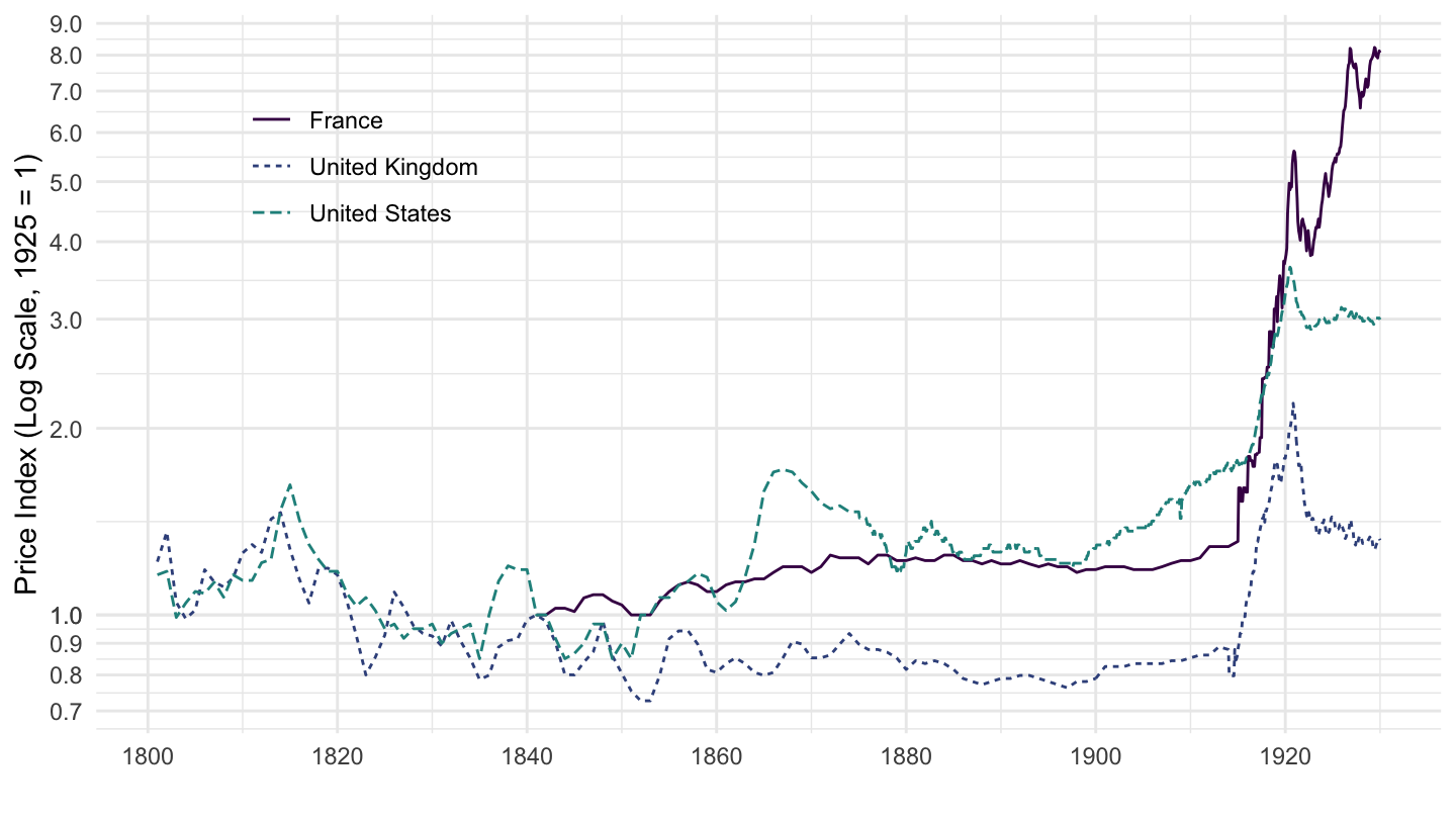
CAN, DNK, NOR
cpi %>%
  filter(iso3c %in% c("CAN", "DNK", "NOR"),
         variable == "CPM",
         date >= as.Date("1800-01-01"),
         date <= as.Date("1930-01-01")) %>%
  left_join(iso3c, by = "iso3c") %>%
  group_by(iso3c) %>%
  mutate(value = 1*value / value[date == as.Date("1840-12-31")]) %>%
  ggplot(.) + geom_line() +
  aes(x = date, y = value, color = Iso3c, linetype = Iso3c) +
  theme_minimal() + xlab("") + ylab("Price Index (Log Scale, 1840 = 1)") +
  scale_x_date(breaks = seq(1800, 2020, 20) %>% paste0("-01-01") %>% as.Date,
               labels = date_format("%Y")) +
  scale_y_log10(breaks = c(seq(0.1, 1, 0.1), seq(1, 10, 1), seq(10, 100, 10)),
                     labels = dollar_format(accuracy = .1, prefix = "")) +
  scale_color_manual(values = viridis(5)[1:4]) +
  theme(legend.position = c(0.3, 0.9),
        legend.title = element_blank())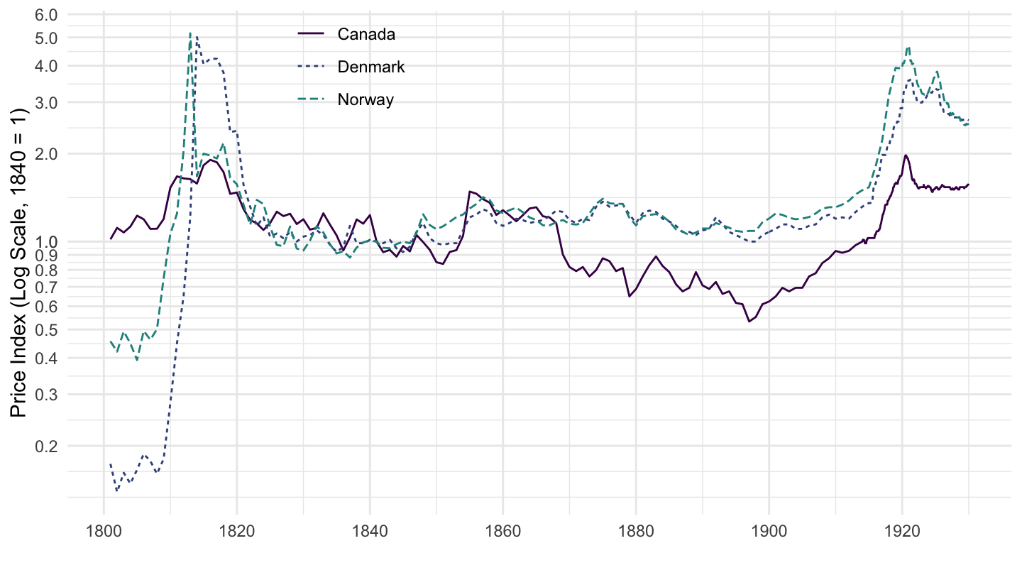
CHE, ESP, ITA, JPN
cpi %>%
  filter(iso3c %in% c("CHE", "ESP", "ITA", "JPN"),
         variable == "CPM",
         date >= as.Date("1800-01-01"),
         date <= as.Date("1930-01-01")) %>%
  left_join(iso3c, by = "iso3c") %>%
  group_by(iso3c) %>%
  mutate(value = 1*value / value[date == as.Date("1869-12-31")]) %>%
  ggplot(.) + geom_line() +
  aes(x = date, y = value, color = Iso3c, linetype = Iso3c) +
  theme_minimal() + xlab("") + ylab("Price Index (1928-06 = 1)") +
  scale_x_date(breaks = seq(1800, 2020, 20) %>% paste0("-01-01") %>% as.Date,
               labels = date_format("%Y")) +
  scale_y_log10(breaks = c(seq(0.1, 1, 0.1), seq(1, 10, 1), seq(10, 100, 10)),
                     labels = dollar_format(accuracy = .1, prefix = "")) +
  scale_color_manual(values = viridis(5)[1:4]) +
  theme(legend.position = c(0.2, 0.80),
        legend.title = element_blank())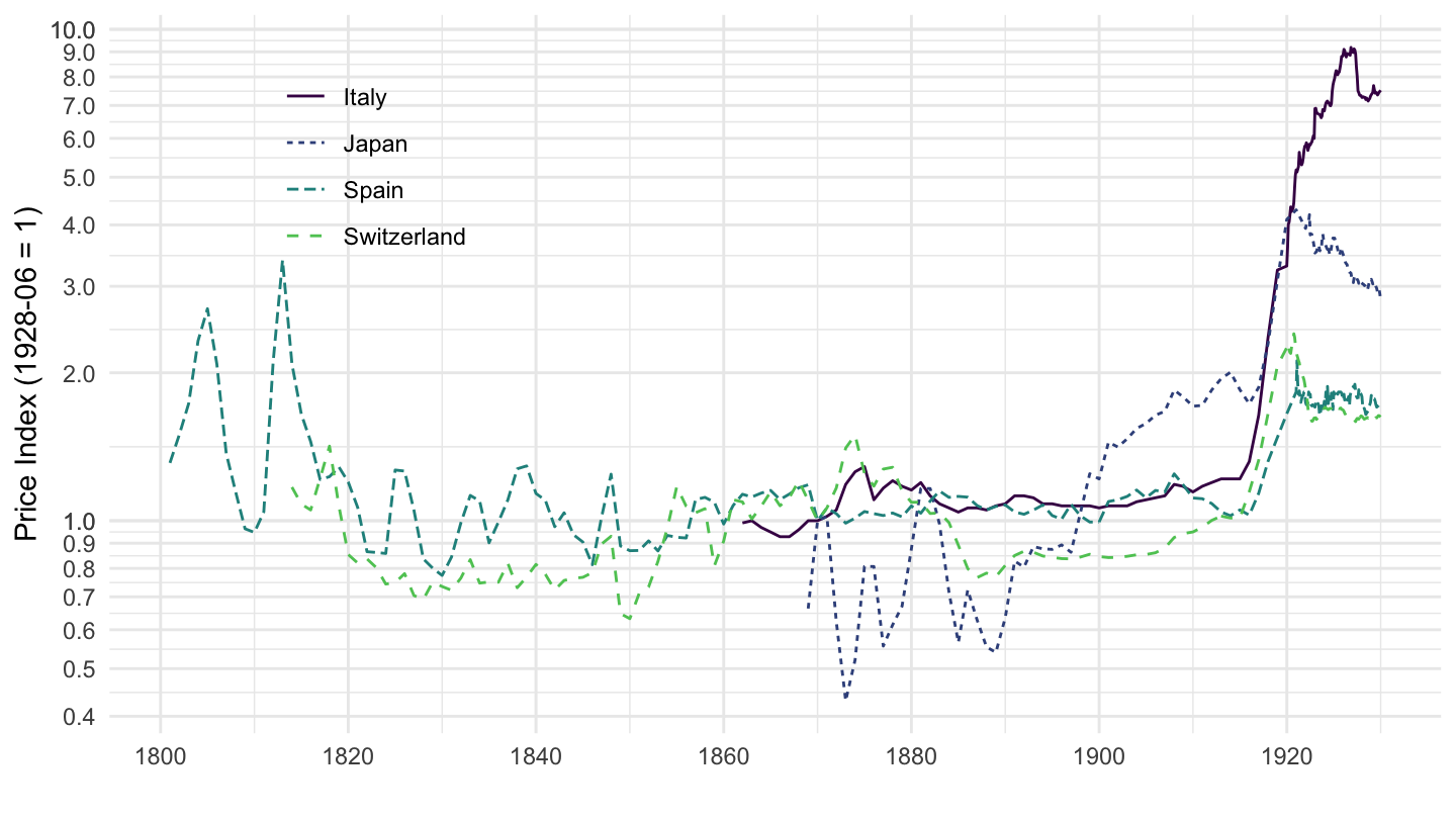
1970-2020
DEU, GBR, USA
cpi %>%
  filter(iso3c %in% c("DEU", "GBR", "USA", "FRA"),
         variable == "CPM",
         date >= as.Date("1970-01-01"),
         date <= as.Date("2020-01-01")) %>%
  left_join(iso3c, by = "iso3c") %>%
  group_by(iso3c) %>%
  mutate(value = 1*value / value[date == as.Date("1970-01-31")]) %>%
  ggplot(.) + geom_line() +
  aes(x = date, y = value, color = Iso3c, linetype = Iso3c) +
  theme_minimal() + xlab("") + ylab("Price Index (Log Scale, 1970 = 1)") +
  scale_x_date(breaks = seq(1925, 2020, 5) %>% paste0("-01-01") %>% as.Date,
               labels = date_format("%y")) +
  scale_y_log10(breaks = c(seq(1, 10, 1), 15, 20, 50),
                     labels = dollar_format(accuracy = 1, prefix = "")) +
  scale_color_manual(values = viridis(5)[1:4]) +
  theme(legend.position = c(0.2, 0.80),
        legend.title = element_blank())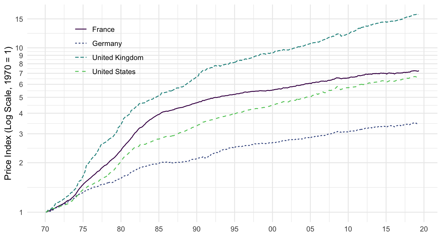
CHE, ESP, ITA, JPN
cpi %>%
  filter(iso3c %in% c("CHE", "ESP", "ITA", "JPN"),
         variable == "CPM",
         date >= as.Date("1970-01-01"),
         date <= as.Date("2020-01-01")) %>%
  left_join(iso3c, by = "iso3c") %>%
  group_by(iso3c) %>%
  mutate(value = 1*value / value[date == as.Date("1970-01-31")]) %>%
  ggplot(.) + geom_line() +
  aes(x = date, y = value, color = Iso3c, linetype = Iso3c) +
  theme_minimal() + xlab("") + ylab("Price Index (1970 = 1)") +
  scale_x_date(breaks = seq(1925, 2020, 5) %>% paste0("-01-01") %>% as.Date,
               labels = date_format("%y")) +
  scale_y_log10(breaks = c(1, 2, 3, 4, 5, 10, 20, 30, 40, 50, 100),
                     labels = dollar_format(accuracy = 1, prefix = "")) +
  scale_color_manual(values = viridis(5)[1:4]) +
  theme(legend.position = c(0.2, 0.80),
        legend.title = element_blank())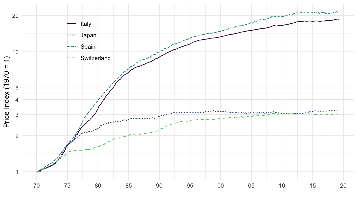
Phillips curves
Great Britain
data_GBR <- cpi %>%
  bind_rows(unr) %>%
  filter(iso3c %in% c("GBR"),
         month(date) == 12,
         variable %in% c("CPM", "UNM")) %>%
  select(variable, date, value) %>%
  spread(variable, value) %>%
  na.omit %>%
  mutate(UNM = UNM / 100,
         CPM = log(CPM),
         CPM = (CPM - lag(CPM, 1)))

data_GBR %>%
  gather(variable, value, -date) %>%
  left_join(variable, by = "variable") %>%
  ggplot(.) +
  geom_line(aes(x = date, y = value, color = Variable, linetype = Variable)) +
  theme_minimal() + xlab("") + ylab("Unemployment, Inflation") +
  scale_x_date(breaks = seq(1700, 2020, 20) %>% paste0("-01-01") %>% as.Date,
               labels = date_format("%Y")) +
  scale_y_continuous(breaks = 0.01*seq(-50, 50, 5),
                     labels = percent_format(accuracy = 1, prefix = "")) +
  scale_color_manual(values = viridis(5)[1:4]) +
  theme(legend.position = c(0.8, 0.2),
        legend.title = element_blank())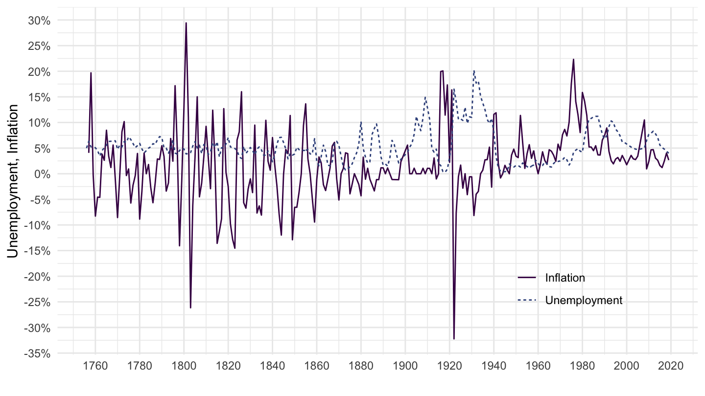
if (knitr::is_html_output()) type <- "html" else type <- "latex"
GBR_post_1971 <- data_GBR %>%
  filter(date >= as.Date("1971-01-01")) %>%
  lm(CPM ~ UNM, data = .)

GBR_pre_1971 <- data_GBR %>%
  filter(date <= as.Date("1971-01-01")) %>%
  lm(CPM ~ UNM, data = .)

GBR_pre_1914 <- data_GBR %>%
  filter(date <= as.Date("1914-01-01")) %>%
  lm(CPM ~ UNM, data = .)

GBR_pre_1914_post_1860 <- data_GBR %>%
  filter(date <= as.Date("1914-01-01"),
         date >= as.Date("1860-01-01")) %>%
  lm(CPM ~ UNM, data = .)

stargazer(GBR_post_1971, GBR_pre_1971, GBR_pre_1914, GBR_pre_1914_post_1860,
          header = F,
          df = F,
          title = "\\textsc{Phillips Curve}",
          column.labels = c("Post 1971", "Pre 1971", "Pre 1920", "1860-1914"),
          dep.var.labels = "Inflation",
          covariate.labels = "Unemployment",
          intercept.bottom = FALSE,
          omit.stat = c("f", "ser", "rsq"),
          omit = "Constant",
          style = "qje",
          notes  = "Data",
          notes.append = FALSE,
          notes.align = "l",
          notes.label = "Note:",
type = type)| Inflation | ||||
| Post 1971 | Pre 1971 | Pre 1920 | 1860-1914 | |
| (1) | (2) | (3) | (4) | |
| Unemployment | -0.686** | -0.581*** | -0.296 | -0.152 |
| (0.269) | (0.137) | (0.259) | (0.098) | |
| N | 45 | 213 | 156 | 52 |
| Adjusted R2 | 0.111 | 0.075 | 0.002 | 0.027 |
| Note: | Data | |||
United States
data_USA <- cpi %>%
  bind_rows(unr) %>%
  filter(iso3c %in% c("USA"),
         month(date) == 12,
         variable %in% c("CPM", "UNM")) %>%
  select(variable, date, value) %>%
  spread(variable, value) %>%
  na.omit %>%
  mutate(UNM = UNM / 100,
         CPM = log(CPM),
         CPM = (CPM - lag(CPM, 1)))

data_USA %>%
  gather(variable, value, -date) %>%
  left_join(variable, by = "variable") %>%
  ggplot(.) +
  geom_line(aes(x = date, y = value, color = Variable, linetype = Variable)) +
  theme_minimal() + xlab("") + ylab("Unemployment, Inflation") +
  scale_x_date(breaks = seq(1700, 2020, 10) %>% paste0("-01-01") %>% as.Date,
               labels = date_format("%Y")) +
  scale_y_continuous(breaks = 0.01*seq(-50, 50, 5),
                     labels = percent_format(accuracy = 1, prefix = "")) +
  scale_color_manual(values = viridis(5)[1:4]) +
  theme(legend.position = c(0.8, 0.9),
        legend.title = element_blank())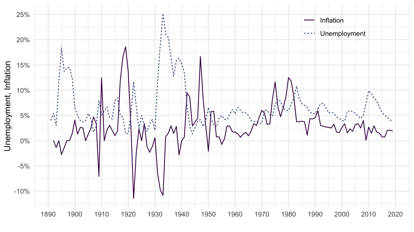
data_USA %>%
  gather(variable, value, -date) %>%
  filter(date <= as.Date("1971-01-01")) %>%
  left_join(variable, by = "variable") %>%
  ggplot(.) +
  geom_line(aes(x = date, y = value, color = Variable, linetype = Variable)) +
  theme_minimal() + xlab("") + ylab("Unemployment, Inflation") +
  scale_x_date(breaks = seq(1700, 2020, 10) %>% paste0("-01-01") %>% as.Date,
               labels = date_format("%Y")) +
  scale_y_continuous(breaks = 0.01*seq(-50, 50, 5),
                     labels = percent_format(accuracy = 1, prefix = "")) +
  scale_color_manual(values = viridis(5)[1:4]) +
  theme(legend.position = c(0.8, 0.9),
        legend.title = element_blank())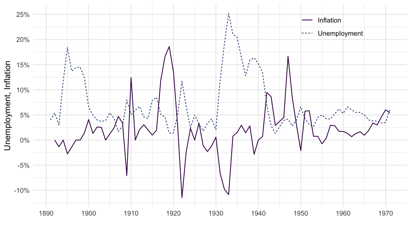
data_USA %>%
  gather(variable, value, -date) %>%
  filter(date >= as.Date("1971-01-01")) %>%
  left_join(variable, by = "variable") %>%
  ggplot(.) +
  geom_line(aes(x = date, y = value, color = Variable, linetype = Variable)) +
  theme_minimal() + xlab("") + ylab("Unemployment, Inflation") +
  scale_x_date(breaks = seq(1700, 2020, 10) %>% paste0("-01-01") %>% as.Date,
               labels = date_format("%Y")) +
  scale_y_continuous(breaks = 0.01*seq(-50, 50, 5),
                     labels = percent_format(accuracy = 1, prefix = "")) +
  scale_color_manual(values = viridis(5)[1:4]) +
  theme(legend.position = c(0.8, 0.9),
        legend.title = element_blank())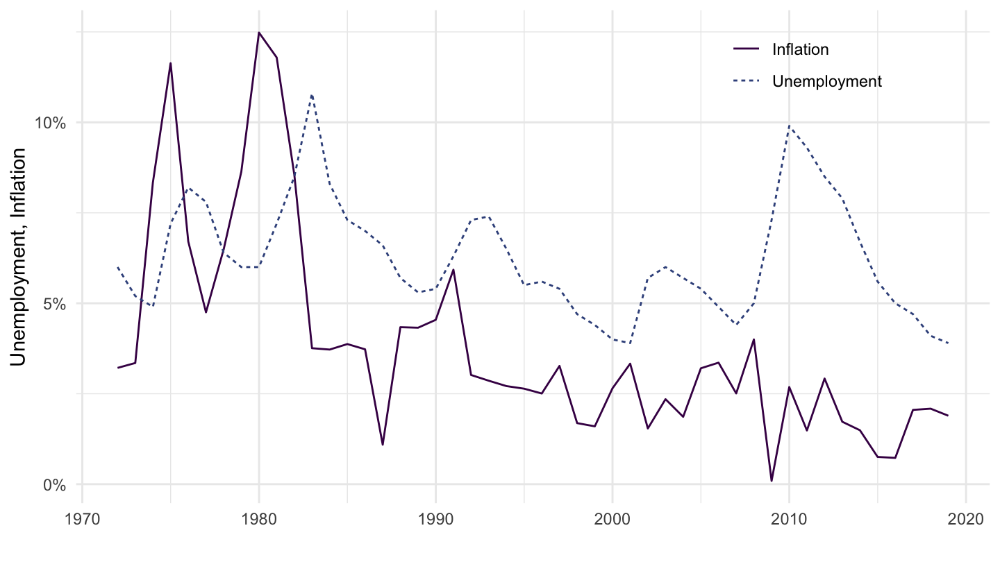
data_USA %>%
  gather(variable, value, -date) %>%
  filter(date >= as.Date("1985-01-01")) %>%
  left_join(variable, by = "variable") %>%
  ggplot(.) +
  geom_line(aes(x = date, y = value, color = Variable, linetype = Variable)) +
  theme_minimal() + xlab("") + ylab("Unemployment, Inflation") +
  scale_x_date(breaks = seq(1700, 2020, 2) %>% paste0("-01-01") %>% as.Date,
               labels = date_format("%Y")) +
  scale_y_continuous(breaks = 0.01*seq(-50, 50, 1),
                     labels = percent_format(accuracy = 1, prefix = "")) +
  scale_color_manual(values = viridis(5)[1:4]) +
  theme(legend.position = c(0.2, 0.9),
        legend.title = element_blank())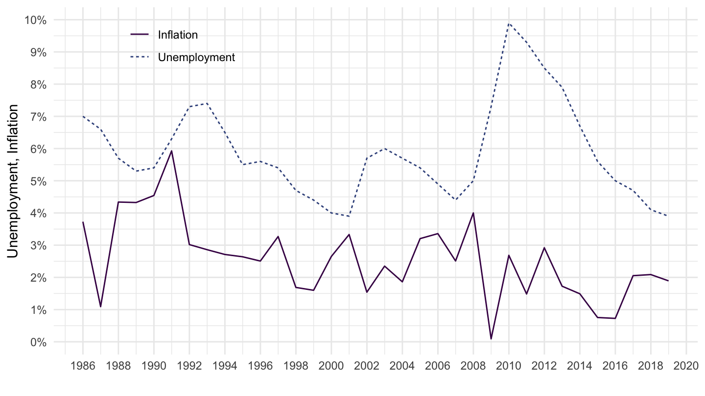
USA_post_1971 <- data_USA %>%
  filter(date >= as.Date("1971-01-01")) %>%
  lm(CPM ~ UNM, data = .)

USA_pre_1971 <- data_USA %>%
  filter(date <= as.Date("1971-01-01")) %>%
  lm(CPM ~ UNM, data = .)

USA_pre_1914 <- data_USA %>%
  filter(date <= as.Date("1914-01-01")) %>%
  lm(CPM ~ UNM, data = .)

stargazer(USA_post_1971, USA_pre_1971, USA_pre_1914,
          header = F,
          df = F,
          title = "\\textsc{Phillips Curve}",
          column.labels = c("Post 1971", "Pre 1971", "Pre 1920"),
          dep.var.labels = "Inflation",
          covariate.labels = "Unemployment",
          intercept.bottom = FALSE,
          omit.stat = c("f", "ser", "rsq"),
          omit = "Constant",
          style = "qje",
          notes  = "Data",
          notes.append = FALSE,
          notes.align = "l",
          notes.label = "Note:",
type = type)| Inflation | |||
| Post 1971 | Pre 1971 | Pre 1920 | |
| (1) | (2) | (3) | |
| Unemployment | 0.283 | -0.471*** | -0.316** |
| (0.261) | (0.099) | (0.151) | |
| N | 48 | 79 | 23 |
| Adjusted R2 | 0.004 | 0.218 | 0.134 |
| Note: | Data | ||
Germany (without 1922, 1923)
data_DEU <- cpi %>%
  bind_rows(unr) %>%
  filter(iso3c %in% c("DEU"),
         month(date) == 12,
         variable %in% c("CPM", "UNM")) %>%
  select(variable, date, value) %>%
  spread(variable, value) %>%
  na.omit %>%
  mutate(UNM = UNM / 100,
         CPM = log(CPM),
         CPM = (CPM - lag(CPM, 1))) %>%
  filter(date != as.Date("1923-12-31"),
         date != as.Date("1922-12-31"))

data_DEU %>%
  gather(variable, value, -date) %>%
  left_join(variable, by = "variable") %>%
  ggplot(.) +
  geom_line(aes(x = date, y = value, color = Variable, linetype = Variable)) +
  theme_minimal() + xlab("") + ylab("Unemployment, Inflation") +
  scale_x_date(breaks = seq(1700, 2020, 20) %>% paste0("-01-01") %>% as.Date,
               labels = date_format("%Y")) +
  scale_y_continuous(breaks = 0.01*seq(-50, 100, 5),
                     labels = percent_format(accuracy = 1, prefix = "")) +
  scale_color_manual(values = viridis(5)[1:4]) +
  theme(legend.position = c(0.7, 0.80),
        legend.title = element_blank())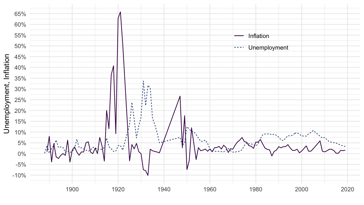
Germany (post 1960)
data_DEU %>%
  filter(date >= as.Date("1954-01-01")) %>%
  gather(variable, value, -date) %>%
  left_join(variable, by = "variable") %>%
  ggplot(.) +
  geom_line(aes(x = date, y = value, color = Variable, linetype = Variable)) +
  theme_minimal() + xlab("") + ylab("Unemployment, Inflation") +
  scale_x_date(breaks = seq(1700, 2020, 5) %>% paste0("-01-01") %>% as.Date,
               labels = date_format("%y")) +
  scale_y_continuous(breaks = 0.01*seq(-50, 100, 1),
                     labels = percent_format(accuracy = 1, prefix = "")) +
  scale_color_manual(values = viridis(5)[1:4]) +
  theme(legend.position = c(0.2, 0.9),
        legend.title = element_blank())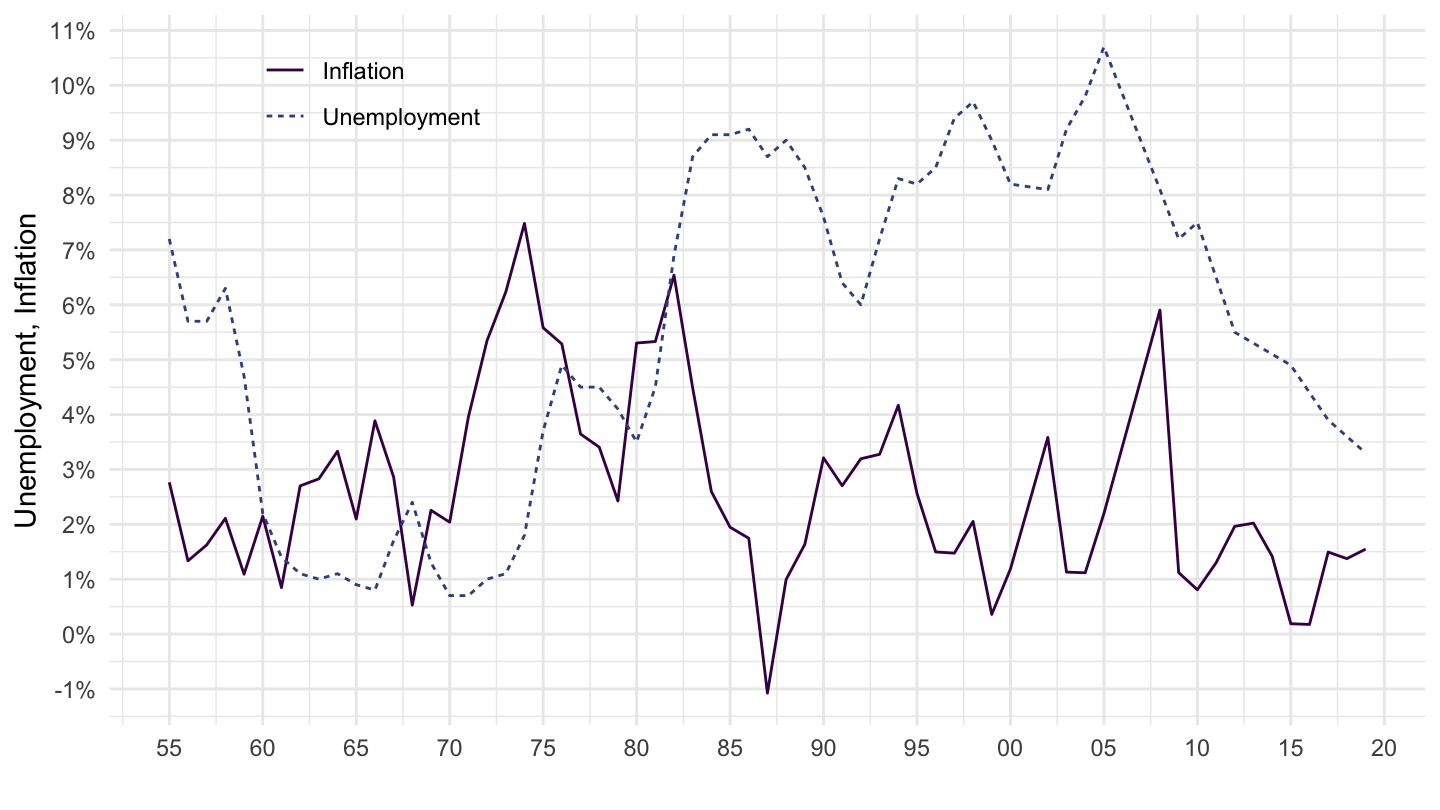
DEU_post_1971 <- data_DEU %>%
  filter(date >= as.Date("1971-01-01")) %>%
  lm(CPM ~ UNM, data = .)

DEU_pre_1971 <- data_DEU %>%
  filter(date <= as.Date("1971-01-01")) %>%
  lm(CPM ~ UNM, data = .)

DEU_pre_1914 <- data_DEU %>%
  filter(date <= as.Date("1914-01-01")) %>%
  lm(CPM ~ UNM, data = .)

stargazer(DEU_post_1971, DEU_pre_1971, DEU_pre_1914,
          header = F,
          df = F,
          title = "\\textsc{Phillips Curve}",
          column.labels = c("Post 1971", "Pre 1971", "Pre 1920"),
          dep.var.labels = "Inflation",
          covariate.labels = "Unemployment",
          intercept.bottom = F,
          omit.stat = c("f", "ser", "rsq"),
          omit = "Constant",
          style = "qje",
          notes = "Data",
          notes.append = F,
          notes.align = "l",
          notes.label = "Note:",
type = type)| Inflation | |||
| Post 1971 | Pre 1971 | Pre 1920 | |
| (1) | (2) | (3) | |
| Unemployment | -0.345*** | -0.433* | -0.587 |
| (0.106) | (0.218) | (0.429) | |
| N | 45 | 73 | 26 |
| Adjusted R2 | 0.178 | 0.039 | 0.034 |
| Note: | Data | ||
France
data_FRA <- cpi %>%
  bind_rows(unr) %>%
  filter(iso3c %in% c("FRA"),
         month(date) == 12,
         variable %in% c("CPM", "UNM")) %>%
  select(variable, date, value) %>%
  spread(variable, value) %>%
  na.omit %>%
  mutate(UNM = UNM / 100,
         CPM = log(CPM),
         CPM = (CPM - lag(CPM, 1)))

data_FRA %>%
  gather(variable, value, -date) %>%
  group_by(variable) %>%
  filter(value <= 2) %>%
  complete(date = seq.Date(min(date), max(date), by = "year")) %>%
  right_join(variable, by = "variable") %>%
  ggplot(.) +
  geom_line(aes(x = date, y = value, color = Variable, linetype = Variable)) +
  theme_minimal() + xlab("") + ylab("Unemployment, Inflation") +
  scale_x_date(breaks = seq(1700, 2020, 20) %>% paste0("-01-01") %>% as.Date,
               labels = date_format("%Y")) +
  scale_y_continuous(breaks = 0.01*seq(-50, 100, 5),
                     labels = percent_format(accuracy = 1, prefix = "")) +
  scale_color_manual(values = viridis(5)[1:4]) +
  theme(legend.position = c(0.4, 0.80),
        legend.title = element_blank())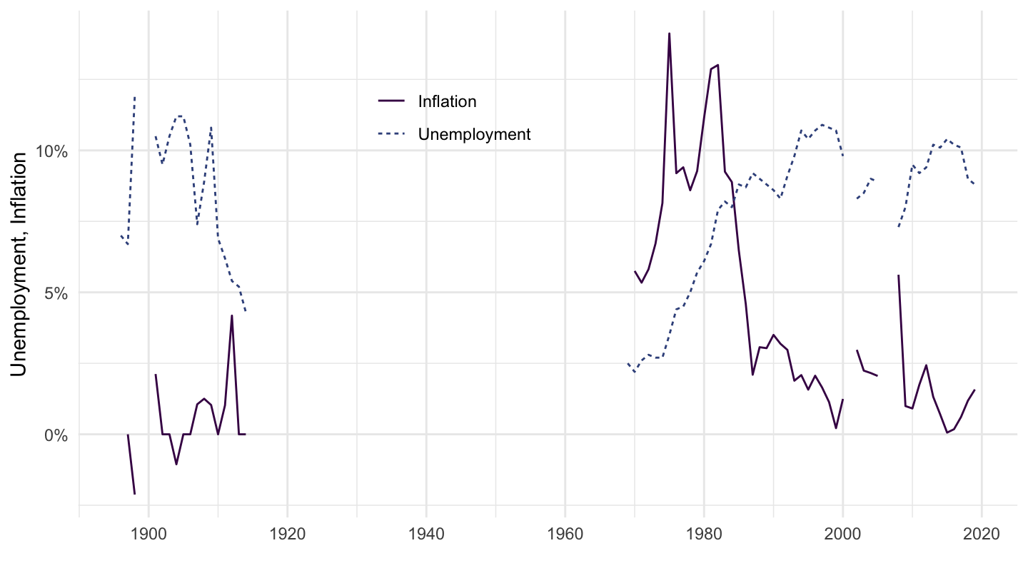
FRA_post_1960 <- data_FRA %>%
  filter(date >= as.Date("1960-01-01")) %>%
  lm(CPM ~ UNM, data = .)

FRA_pre_1913 <- data_FRA %>%
  filter(date <= as.Date("1913-01-01")) %>%
  lm(CPM ~ UNM, data = .)

FRA_all <- data_FRA %>%
  lm(CPM ~ UNM, data = .)

stargazer(FRA_post_1960, FRA_pre_1913, FRA_all,
          header = F,
          df = F,
          title = "\\textsc{Phillips Curve}",
          column.labels = c("Post 1960", "Pre 1913", "All"),
          dep.var.labels = "Inflation",
          covariate.labels = "Unemployment",
          intercept.bottom = F,
          omit.stat = c("f", "ser", "rsq"),
          omit = "Constant",
          style = "qje",
          notes = "Data",
          notes.append = F,
          notes.align = "l",
          notes.label = "Note:",
type = type)| Inflation | |||
| Post 1960 | Pre 1913 | All | |
| (1) | (2) | (3) | |
| Unemployment | -10.247** | -0.294* | -8.229** |
| (4.373) | (0.151) | (3.350) | |
| N | 48 | 15 | 64 |
| Adjusted R2 | 0.087 | 0.165 | 0.074 |
| Note: | Data | ||
Denmark
data_DNK <- cpi %>%
  bind_rows(unr) %>%
  filter(iso3c %in% c("DNK"),
         month(date) == 12,
         variable %in% c("CPM", "UNM")) %>%
  select(variable, date, value) %>%
  spread(variable, value) %>%
  na.omit %>%
  mutate(UNM = UNM / 100,
         CPM = log(CPM),
         CPM = (CPM - lag(CPM, 1)))

data_DNK %>%
  gather(variable, value, -date) %>%
  right_join(variable, by = "variable") %>%
  ggplot(.) +
  geom_line(aes(x = date, y = value, color = Variable, linetype = Variable)) +
  theme_minimal() + xlab("") + ylab("Unemployment, Inflation") +
  scale_x_date(breaks = seq(1700, 2020, 20) %>% paste0("-01-01") %>% as.Date,
               labels = date_format("%Y")) +
  scale_y_continuous(breaks = 0.01*seq(-50, 50, 5),
                     labels = percent_format(accuracy = 1, prefix = "")) +
  scale_color_manual(values = viridis(5)[1:4]) +
  theme(legend.position = c(0.7, 0.80),
        legend.title = element_blank())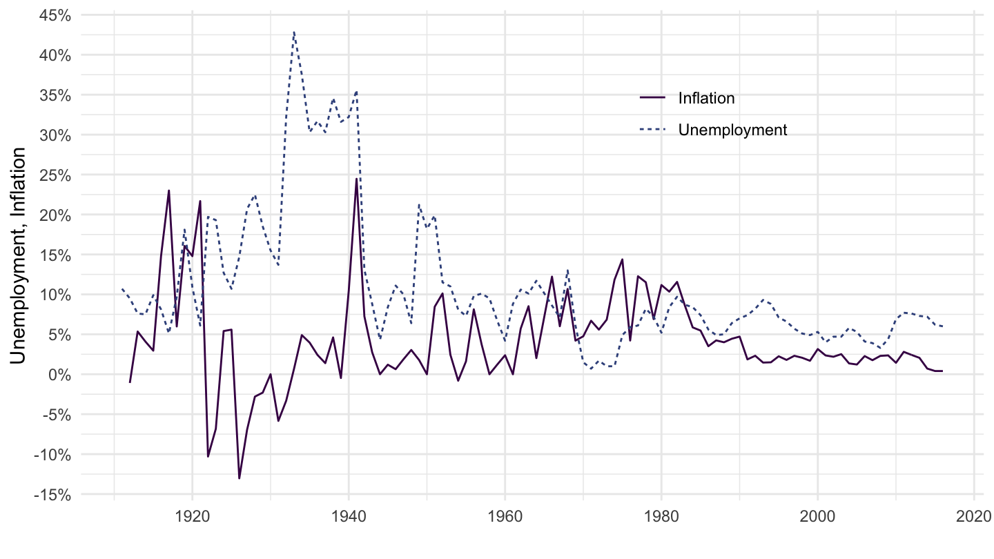
if (knitr::is_html_output()) type <- "html" else type <- "latex"
DNK_post_1971 <- data_DNK %>%
  filter(date >= as.Date("1971-01-01")) %>%
  lm(CPM ~ UNM, data = .)

DNK_pre_1971 <- data_DNK %>%
  filter(date <= as.Date("1971-01-01")) %>%
  lm(CPM ~ UNM, data = .)

DNK_pre_1940 <- data_DNK %>%
  filter(date <= as.Date("1940-01-01")) %>%
  lm(CPM ~ UNM, data = .)

DNK_pre_1930 <- data_DNK %>%
  filter(date <= as.Date("1930-01-01")) %>%
  lm(CPM ~ UNM, data = .)

stargazer(DNK_post_1971, DNK_pre_1971, DNK_pre_1940, DNK_pre_1930,
          header = F,
          df = F,
          title = "\\textsc{Phillips Curve}",
          column.labels = c("Post 1971", "Pre 1971", "Pre 1940", "Pre 1930"),
          dep.var.labels = "Inflation",
          covariate.labels = "Unemployment",
          intercept.bottom = FALSE,
          omit.stat = c("f", "ser", "rsq"),
          omit = "Constant",
          style = "qje",
          notes  = "Data",
          notes.append = FALSE,
          notes.align = "l",
          notes.label = "Note:",
type = type)| Inflation | ||||
| Post 1971 | Pre 1971 | Pre 1940 | Pre 1930 | |
| (1) | (2) | (3) | (4) | |
| Unemployment | -0.013 | -0.072 | -0.236 | -1.251*** |
| (0.282) | (0.094) | (0.148) | (0.345) | |
| N | 45 | 59 | 29 | 19 |
| Adjusted R2 | -0.023 | -0.007 | 0.052 | 0.403 |
| Note: | Data | |||
Hyperinflation in Weimar
Germany, Unnited Kingdom
cpi %>%
  filter(iso3c %in% c("DEU", "GBR", "USA"),
         variable == "CPM",
         date >= as.Date("1900-01-01"),
         date <= as.Date("1940-01-01")) %>%
  left_join(iso3c, by = "iso3c") %>%
  group_by(iso3c) %>%
  mutate(value = 1*value / value[date == as.Date("1900-12-31")]) %>%
  ggplot(.) +
  geom_line(aes(x = date, y = value, color = Iso3c)) +
  theme_minimal() + xlab("") + ylab("Price Index (Log Scale, 1900 = 1)") +
  geom_image(data = . %>%
               filter(date == as.Date("1922-12-31")) %>%
               mutate(image = paste0("../../icon/flag/", str_to_lower(gsub(" ", "-", Iso3c)), ".png")),
             aes(x = date, y = value, image = image), asp = 1.5) +
  scale_x_date(breaks = seq(1800, 2020, 5) %>% paste0("-01-01") %>% as.Date,
               labels = date_format("%Y")) +
  scale_y_log10(breaks = 10^seq(0, 20, 1),
                labels = dollar_format(accuracy = 1, prefix = "")) +
  scale_color_manual(values = c("#000000", "#6E82B5", "#B22234")) +
  theme(legend.position = c(0.2, 0.80),
        legend.title = element_blank())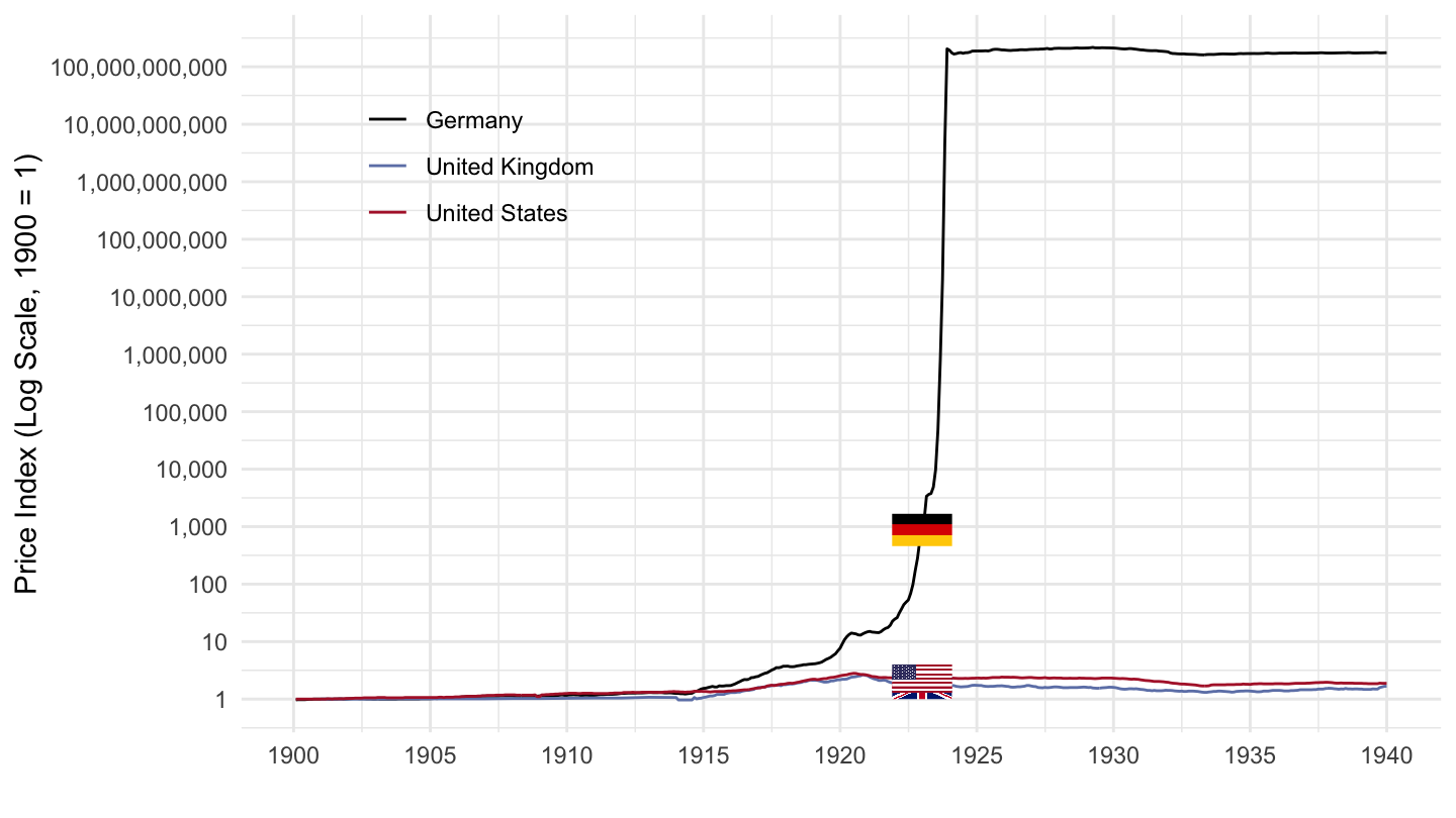
cpi %>%
  filter(iso3c %in% c("DEU", "GBR"),
         variable == "CPM",
         date >= as.Date("1900-01-01"),
         date <= as.Date("1940-01-01")) %>%
  left_join(iso3c, by = "iso3c") %>%
  group_by(iso3c) %>%
  mutate(value = 1*value / value[date == as.Date("1900-12-31")]) %>%
  ggplot(.) +
  geom_line(aes(x = date, y = value, color = Iso3c)) +
  theme_minimal() + xlab("") + ylab("Price Index (Log Scale, 1900 = 1)") +
  geom_image(data = . %>%
               filter(date == as.Date("1922-12-31")) %>%
               mutate(image = paste0("../../icon/flag/", str_to_lower(gsub(" ", "-", Iso3c)), ".png")),
             aes(x = date, y = value, image = image), asp = 1.5) +
  scale_x_date(breaks = seq(1800, 2020, 5) %>% paste0("-01-01") %>% as.Date,
               labels = date_format("%Y")) +
  scale_y_log10(breaks = 10^seq(0, 20, 1),
                labels = dollar_format(accuracy = 1, prefix = "")) +
  scale_color_manual(values = c("#000000", "#6E82B5", "#B22234")) +
  theme(legend.position = c(0.2, 0.80),
        legend.title = element_blank())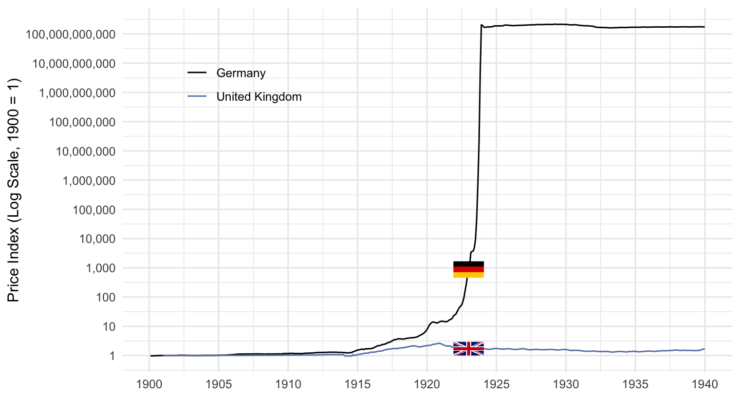
Metadata
cpi_info %>%
  select(Ticker, Name, Metadata) %>%
  {if (is_html_output()) datatable(., filter = 'top', rownames = F) else .}
Econ 102
Deflation during the Great Depression
cpi %>%
  filter(iso3c %in% c("DEU", "GBR", "USA", "FRA"),
         variable == "CPM",
         date >= as.Date("1925-01-01"),
         date <= as.Date("1940-01-01")) %>%
  left_join(iso3c, by = "iso3c") %>%
  group_by(iso3c) %>%
  mutate(value = 1*value / value[date == as.Date("1925-01-31")]) %>%
  ggplot(.) + geom_line() +
  aes(x = date, y = value, color = Iso3c, linetype = Iso3c) +
  theme_minimal() + xlab("") + ylab("Price Index (Log Scale, 1925 = 1)") +
  scale_x_date(breaks = seq(1925, 2020, 1) %>% paste0("-01-01") %>% as.Date,
               labels = date_format("%y")) +
  scale_y_log10(breaks = seq(0.1, 3, 0.1),
                labels = dollar_format(accuracy = .1, prefix = "")) +
  scale_color_manual(values = viridis(5)[1:4]) +
  theme(legend.position = c(0.4, 0.90),
        legend.title = element_blank(),
        legend.direction = "horizontal")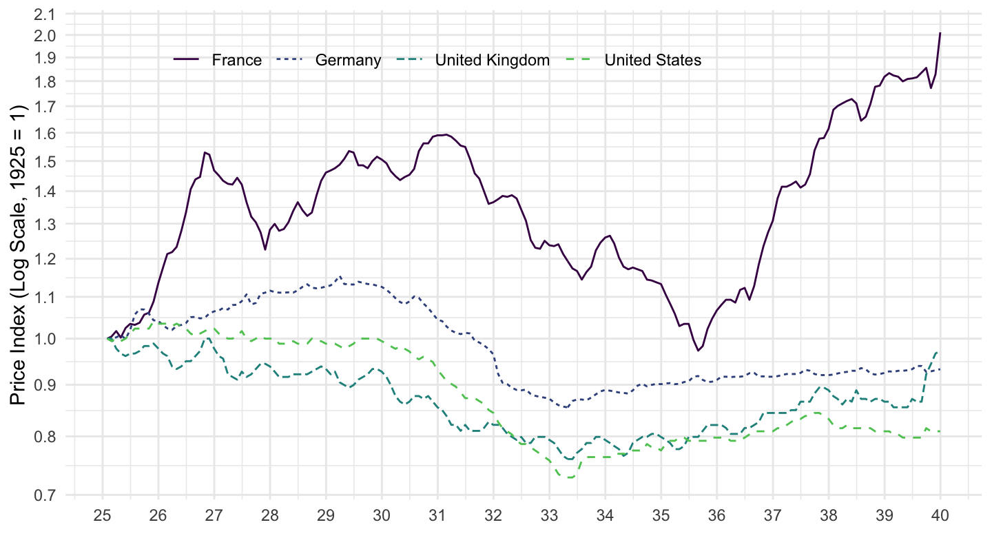
Figure 4: Deflation during the Great Depression
Inflation in Italy, Japan, Spain, and Switzerland (1925-1970)
cpi %>%
  filter(iso3c %in% c("ESP", "ITA", "JPN", "FRA", "DEU"),
         variable == "CPM",
         date >= as.Date("1925-01-01"),
         date <= as.Date("1970-01-01")) %>%
  left_join(iso3c, by = "iso3c") %>%
  group_by(iso3c) %>%
  mutate(value = 1*value / value[date == as.Date("1925-01-31")]) %>%
  ggplot(.) + geom_line() +
  aes(x = date, y = value, color = Iso3c, linetype = Iso3c) +
  theme_minimal() + xlab("") + ylab("Price Index (1925 = 1)") +
  scale_x_date(breaks = seq(1925, 2020, 5) %>% paste0("-01-01") %>% as.Date,
               labels = date_format("%y")) +
  scale_y_log10(breaks = c(1, 2, 3, 4, 5, 10, 20, 30, 40, 50, 100, 200),
                     labels = dollar_format(accuracy = 1, prefix = "")) +
  scale_color_manual(values = viridis(6)[1:5]) +
  theme(legend.position = c(0.2, 0.80),
        legend.title = element_blank())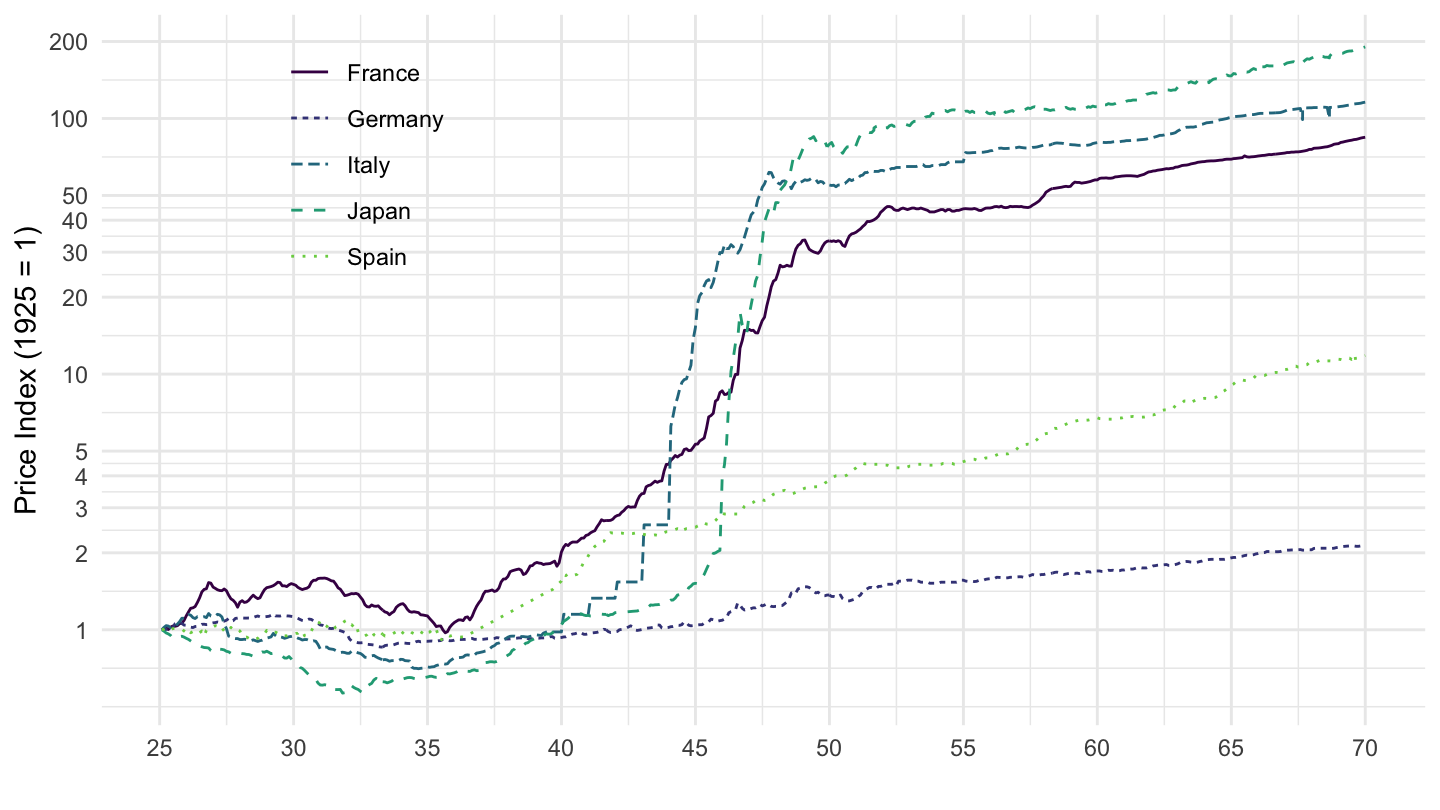
Figure 5: Inflation in Italy, Japan, Spain, and Switzerland (1925-1970)