Production in industry - quarterly data

Data - Eurostat

Author

François Geerolf

Info

Last observation: Quarterly: 2026Q2 (N = 10,141)

First observation: Quarterly: 1953Q1 (N = 9)

Last data update: 09 aoû 2026, 10:35. Last compile: 09 aoû 2026, 17:06

Structure

Industrial Production

France, Germany, Italy

Code

sts_inpr_q |>
  filter(nace_r2 == "C",
         unit == "I15",
         geo %in% c("FR", "DE", "IT"),
         s_adj == "SCA") |>
  select(geo, Geo, time, values) |>
  group_by(geo) |>
  mutate(values = 100*values/values[time == "1997Q1"]) |>
  
  mutate(Geo = ifelse(geo == "DE", "Germany", Geo)) |>
  quarter_to_date() |>
  left_join(colors, by = c("Geo" = "country")) |>
  ggplot() + ylab("Industrial Production") + xlab("") + theme_minimal() +
  geom_line(aes(x = date, y = values, color = color)) +
  scale_color_identity() + add_flags +
  scale_color_manual(values = c("#0055a4", "#000000", "#008c45")) +
  scale_x_date(breaks = seq(1920, 2100, 2) |> paste0("-01-01") |> as.Date(),
               labels = date_format("%Y")) +
  geom_image(data = tibble(date = rep(as.Date("2022-01-01"), 3),
                           value = c(110, 140, 85),
                           image = c("~/iCloud/bib/flags/france.png",
                                     "~/iCloud/bib/flags/germany.png",
                                     "~/iCloud/bib/flags/italy.png")),
             aes(x = date, y = value, image = image), asp = 1.5) +
  theme(legend.position = "none") +
  scale_y_log10(breaks = seq(-60, 300, 10))

Year-on-Year Growth, France

Code

sts_inpr_q |>
  filter(geo == "FR",
         nace_r2 == "C",
         unit == "PCH_SM",
         s_adj == "CA") |>
  quarter_to_date() |>
  mutate(values = values/100) |>
  ggplot() + geom_line(aes(x = date, y = values)) +
  theme_minimal() +
  scale_x_date(breaks = as.Date(paste0(seq(1990, 2100, 5), "-01-01")),
               labels = date_format("%Y")) +
  xlab("") + ylab("Industrial production, YoY growth (France)") +
  scale_y_continuous(labels = scales::percent_format(accuracy = 1)) +
  geom_hline(yintercept = 0, linetype = "dashed", color = "black")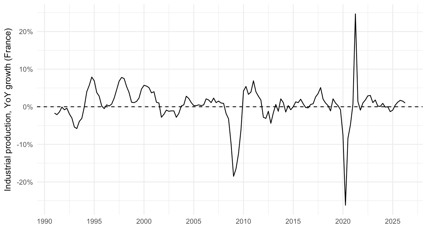

Main Industrial Groupings, France

Code

sts_inpr_q |>
  filter(geo == "FR",
         nace_r2 %in% c("MIG_CAG", "MIG_COG", "MIG_ING"),
         unit == "I15",
         s_adj == "SCA") |>
  quarter_to_date() |>
  ggplot() + geom_line(aes(x = date, y = values, color = Nace_r2)) +
  theme_minimal() +
  theme(legend.position = c(0.3, 0.85),
        legend.title = element_blank()) +
  scale_x_date(breaks = as.Date(paste0(seq(1990, 2100, 5), "-01-01")),
               labels = date_format("%Y")) +
  xlab("") + ylab("Production index, 2015 = 100 (France)")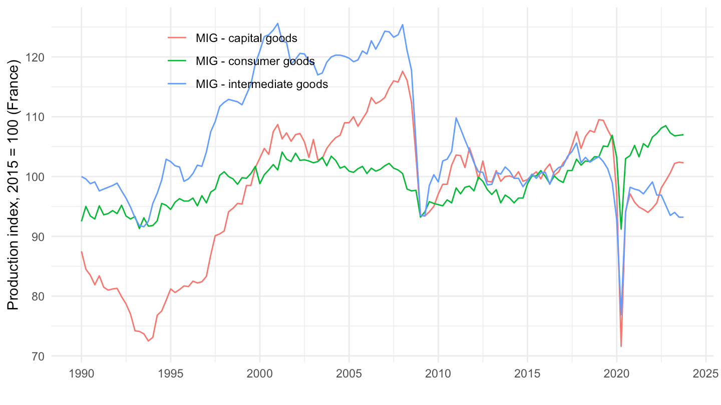

Latest Quarter Snapshot: Industrial Production Growth

Code

latest_q <- sts_inpr_q |>
  filter(nace_r2 == "C", unit == "PCH_SM", s_adj == "CA",
         geo %in% c("FR", "DE", "IT", "ES", "PL"), !is.na(values)) |>
  summarise(m = max(time)) |>
  pull(m)

sts_inpr_q |>
  filter(nace_r2 == "C",
         unit == "PCH_SM",
         s_adj == "CA",
         geo %in% c("FR", "DE", "IT", "ES", "PL"),
         time == latest_q) |>
  select(Geo, values) |>
  arrange(desc(values)) |>
  print_table_conditional()

Geo	values
Poland	3.2
Spain	1.9
France	1.0
Italy	0.6
Germany	-1.0