
Last observation: sept. 2026 (N = 18)
First observation: janv. 1980 (N = 4)
Last data update: 18 oct. 2026, 23:19
Last compile: 24 oct. 2026, 01:42
sts_copi_m |>
  filter(geo %in% c("ES", "AT", "PT", "NL"),
         indic_bt == "COST",
         unit == "I21") |>
  month_to_date() |>

  add_flag_color("Geo") |>
  ggplot() + geom_line(aes(x = date, y = values, color = color)) +
  theme_minimal() + scale_color_identity() + add_flags +
  scale_x_date(breaks = as.Date(paste0(seq(1980, 2100, 5), "-01-01")),
               labels = date_format("%Y")) +
  xlab("") + ylab("Construction cost, new residential buildings (2021 = 100)")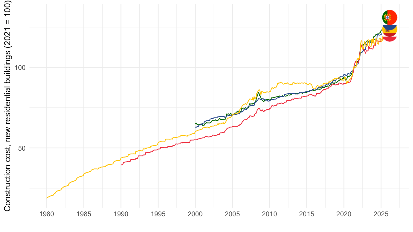
sts_copi_m |>
  filter(geo == "ES",
         unit == "PCH_SM") |>
  month_to_date() |>

  mutate(values = values/100) |>
  ggplot() + geom_line(aes(x = date, y = values, color = Indic_bt)) +
  theme_minimal() +
  scale_x_date(breaks = as.Date(paste0(seq(1980, 2100, 5), "-01-01")),
               labels = date_format("%Y")) +
  theme(legend.position = c(0.2, 0.85),
        legend.title = element_blank()) +
  xlab("") + ylab("Year-on-year change") +
  scale_y_continuous(labels = scales::percent_format(accuracy = 1)) +
  geom_hline(yintercept = 0, linetype = "dashed", color = "black")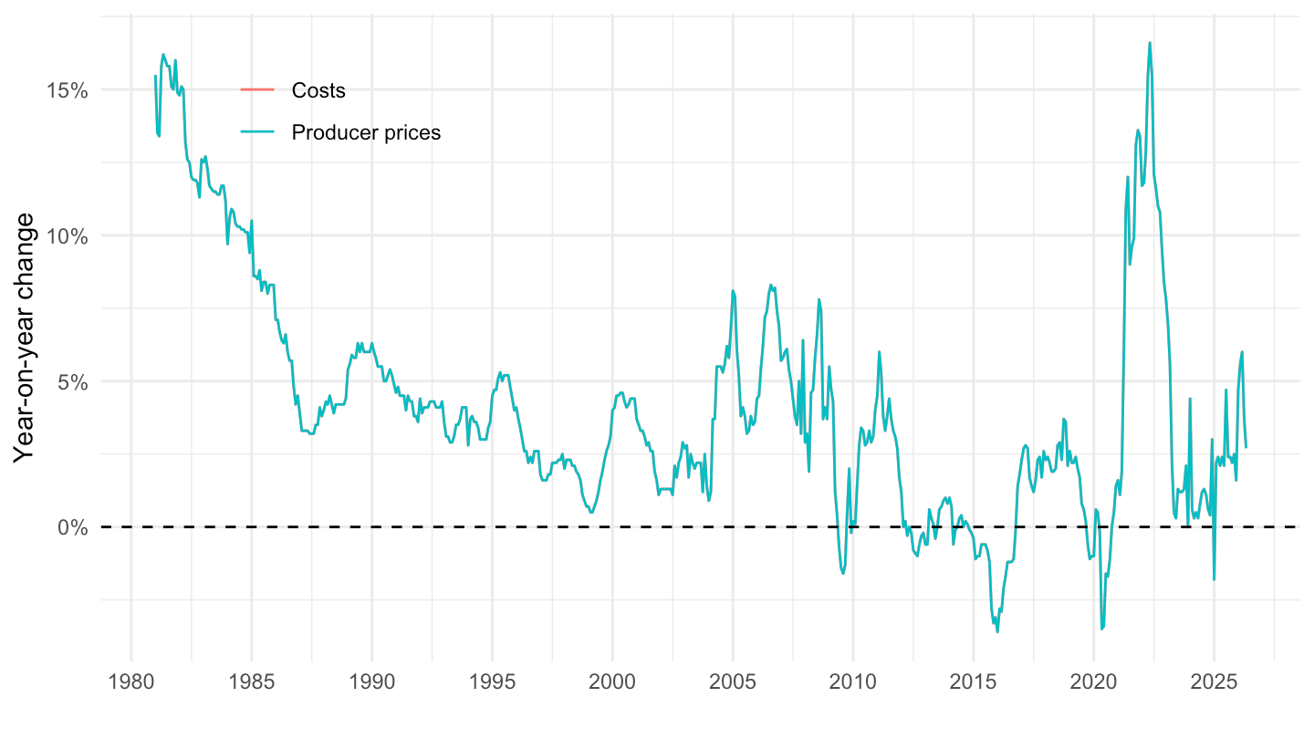
latest_m <- sts_copi_m |>
  filter(geo == "ES",
         indic_bt == "COST",
         unit == "PCH_SM",
         !is.na(values)) |>
  summarise(m = max(time)) |>
  pull(m)

sts_copi_m |>
  filter(unit == "PCH_SM",
         time == latest_m) |>
  mutate(values = values/100) |>
  select(Geo, Indic_bt, values) |>
  spread(Indic_bt, values) |>
  arrange(-Costs) |>
print_table_conditional()| Geo | Costs | Producer prices |
|---|---|---|
| Türkiye | 0.283 | 0.283 |
| Portugal | 0.065 | 0.065 |
| Austria | 0.052 | 0.052 |
| Netherlands | 0.050 | 0.050 |
| Lithuania | 0.048 | 0.048 |
| Norway | 0.044 | 0.044 |
| Finland | 0.033 | 0.033 |
| Spain | 0.033 | 0.033 |
| Ireland | NA | 0.034 |
| Italy | NA | 0.023 |
| Poland | NA | 0.063 |