House sales index of value of transactions (2015=100) - annual data - prc_hpi_hsvq

Data - Eurostat

Info

Last observation: Quarterly: 2026Q1 (N = 224)

First observation: Quarterly: 2006Q1 (N = 13)

Last data update: 23 jul 2026, 22:11. Last compile: 24 jul 2026, 03:44

Structure

freq

unit

geo

purchase

France: New vs. Existing Dwellings

prc_hpi_hsvq %>%
  filter(geo == "FR",
         unit == "I25_Q",
         purchase %in% c("DW_NEW", "DW_EXST")) %>%
  quarter_to_date %>%

  ggplot + geom_line(aes(x = date, y = values, color = Purchase)) +
  theme_minimal() +
  scale_x_date(breaks = as.Date(paste0(seq(2005, 2100, 2), "-01-01")),
               labels = date_format("%Y")) +
  theme(legend.position = c(0.25, 0.85),
        legend.title = element_blank()) +
  xlab("") + ylab("House sales index (2025=100)")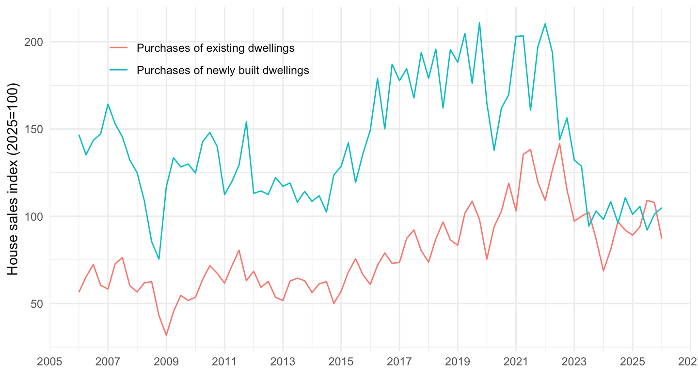

Annual Rate of Change: France, Spain, Netherlands

prc_hpi_hsvq %>%
  filter(geo %in% c("FR", "ES", "NL"),
         unit == "RCH_A",
         purchase == "TOTAL") %>%
  quarter_to_date %>%

  left_join(colors, by = c("Geo" = "country")) %>%
  mutate(values = values/100) %>%
  ggplot + geom_line(aes(x = date, y = values, color = color)) +
  theme_minimal() + scale_color_identity() + add_3flags +
  scale_x_date(breaks = as.Date(paste0(seq(2005, 2100, 2), "-01-01")),
               labels = date_format("%Y")) +
  theme(legend.position = c(0.2, 0.85),
        legend.title = element_blank()) +
  xlab("") + ylab("House sales index, annual rate of change") +
  scale_y_continuous(labels = scales::percent_format(accuracy = 1)) +
  geom_hline(yintercept = 0, linetype = "dashed", color = "black")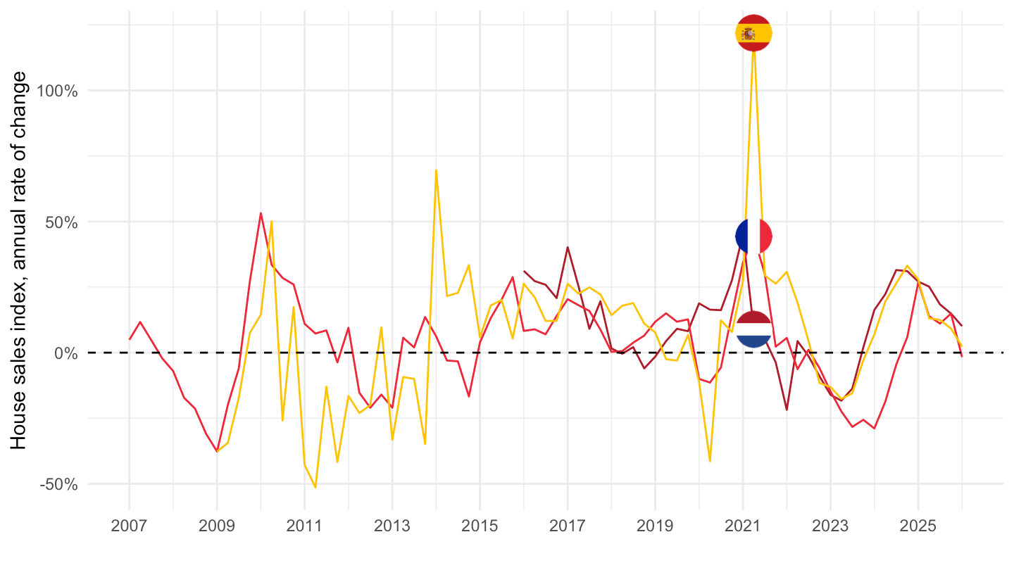

Latest Quarter by Country

latest_q <- prc_hpi_hsvq %>%
  filter(unit == "I25_Q",
         purchase == "TOTAL",
         !is.na(values)) %>%
  summarise(m = max(time)) %>%
  pull(m)

prc_hpi_hsvq %>%
  filter(unit == "I25_Q",
         purchase == "TOTAL",
         time == latest_q) %>%
  mutate(values = round(values, 1)) %>%
  select(Geo, values) %>%
  arrange(-values) %>%
  print_table_conditional()

Geo	values
Cyprus	101.6
Slovenia	101.6
Hungary	99.3
Malta	99.3
Lithuania	99.1
Denmark	98.5
Spain	97.6
Portugal	95.9
Netherlands	94.2
Belgium	92.4
Austria	89.0
France	88.7
Bulgaria	80.8
Luxembourg	80.8
Finland	77.3
Ireland	74.0
Croatia	68.5
Norway	61.5

Purchase Total

France, Spain, Austria

prc_hpi_hsvq %>%
  filter(geo %in% c("FR", "ES", "AT"),
         unit == "I25_Q",
         purchase == "TOTAL") %>%
  quarter_to_date %>%
  
  ggplot() + geom_line() + theme_minimal() +
  aes(x = date, y = values, color = Geo, linetype = Geo) +
  scale_color_manual(values = viridis(4)[1:3]) +
  scale_x_date(breaks = seq(1920, 2100, 1) %>% paste0("-01-01") %>% as.Date,
               labels = date_format("%Y")) +
  theme(legend.position = c(0.35, 0.9),
        legend.title = element_blank()) +
  scale_y_log10(breaks = seq(-100, 300, 10)) +
  ylab("House Price Index") + xlab("")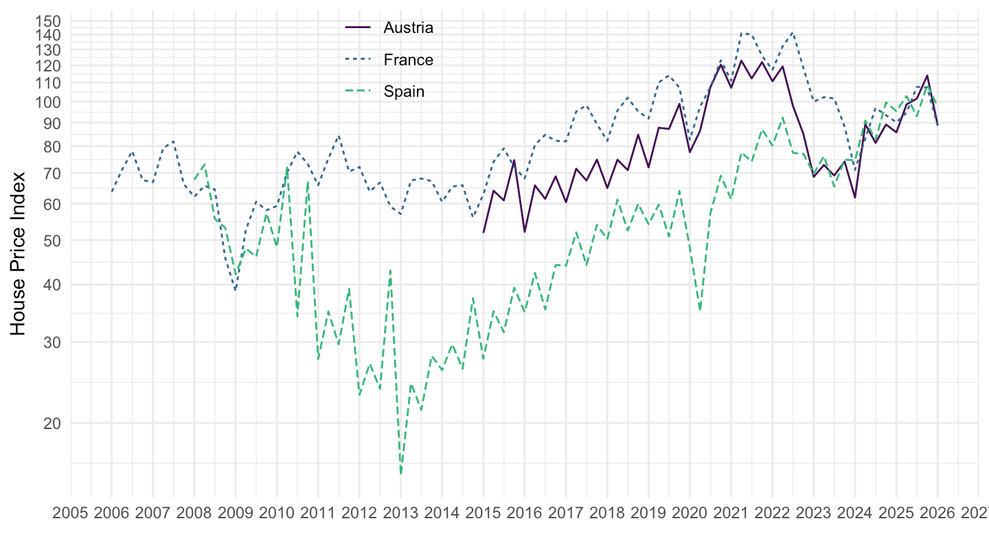

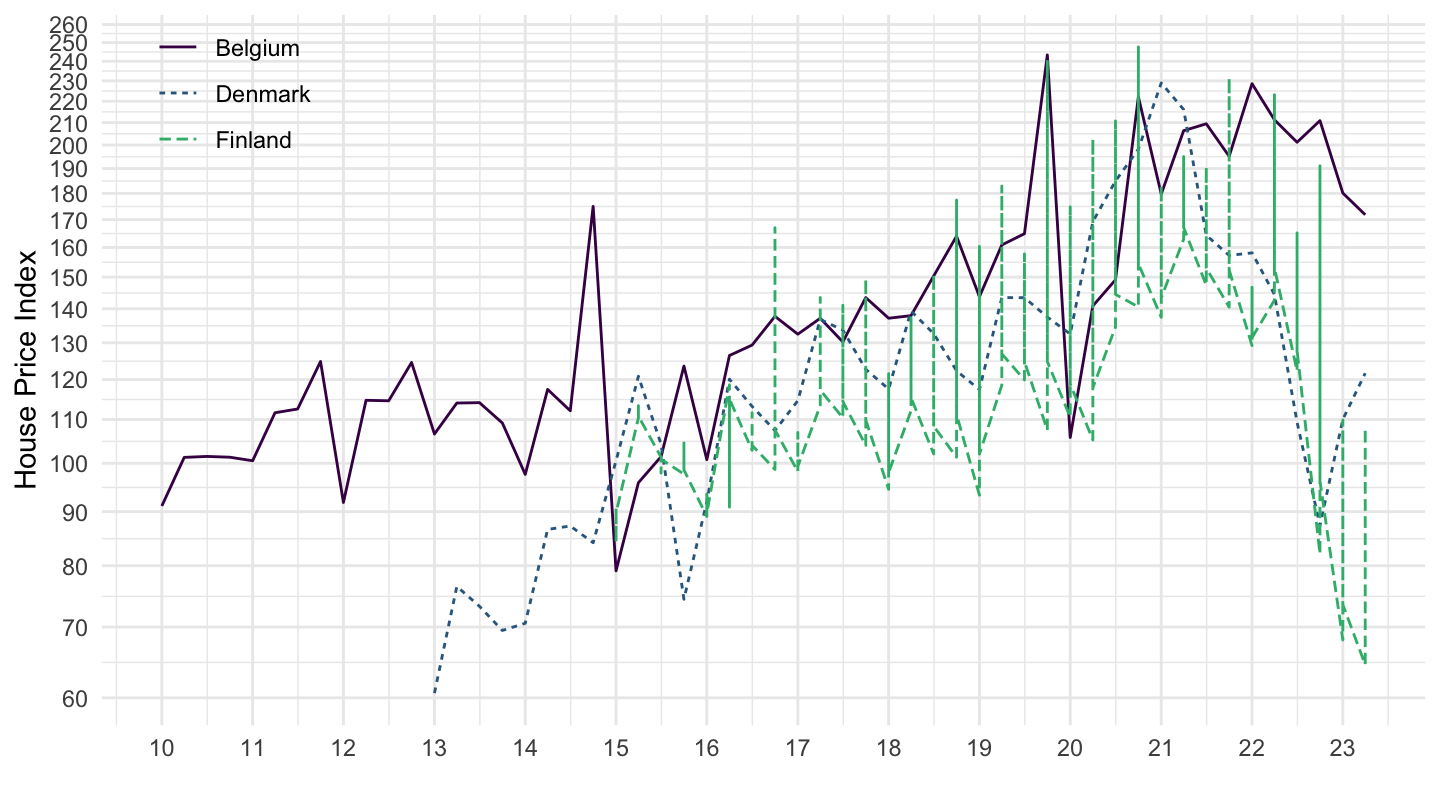
Belgium, Denmark, Finland

prc_hpi_hsvq %>%
  filter(geo %in% c("BE", "DK", "FI"),
         unit == "I25_Q",
         purchase == "TOTAL") %>%
  quarter_to_date %>%
  
  ggplot() + geom_line() + theme_minimal() +
  aes(x = date, y = values, color = Geo, linetype = Geo) +
  scale_color_manual(values = viridis(4)[1:3]) +
  scale_x_date(breaks = seq(1920, 2100, 1) %>% paste0("-01-01") %>% as.Date,
               labels = date_format("%Y")) +
  theme(legend.position = c(0.1, 0.9),
        legend.title = element_blank()) +
  scale_y_log10(breaks = seq(-100, 300, 10)) +
  ylab("House Price Index") + xlab("")