Financial balance sheets - nasa_10_f_bs

Data - Eurostat

Info

Last observation: Annual: 2025 (N = 349,984)

First observation: Annual: 1990 (N = 7,676)

Last data update: 23 jul 2026, 22:27. Last compile: 24 jul 2026, 03:04

Structure

freq

unit

co_nco

sector

finpos

na_item

geo

Net Financial Worth Over Time (% of GDP)

Total Economy: France, Germany, Italy, Spain

nasa_10_f_bs %>%
  filter(geo %in% c("FR", "DE", "IT", "ES"),
         sector == "S1",
         co_nco == "CO",
         na_item == "BF90",
         unit == "PC_GDP") %>%
  year_to_date %>%
  left_join(colors, by = c("Geo" = "country")) %>%
  mutate(values = values/100) %>%
  ggplot + geom_line(aes(x = date, y = values, color = color)) +
  theme_minimal() + scale_color_identity() + add_4flags +
  scale_x_date(breaks = as.Date(paste0(seq(1990, 2100, 5), "-01-01")),
               labels = date_format("%Y")) +
  xlab("") + ylab("Net financial worth, total economy (% of GDP)") +
  scale_y_continuous(labels = scales::percent_format(accuracy = 1)) +
  geom_hline(yintercept = 0, linetype = "dashed", color = "black")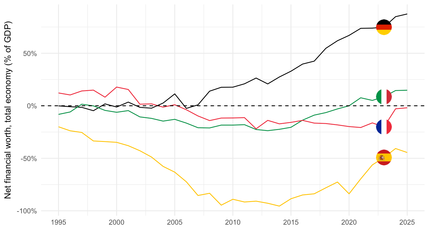

Households: France, Germany, Italy, Spain

nasa_10_f_bs %>%
  filter(geo %in% c("FR", "DE", "IT", "ES"),
         sector == "S14_S15",
         co_nco == "CO",
         na_item == "BF90",
         unit == "PC_GDP") %>%
  year_to_date %>%
  left_join(colors, by = c("Geo" = "country")) %>%
  mutate(values = values/100) %>%
  ggplot + geom_line(aes(x = date, y = values, color = color)) +
  theme_minimal() + scale_color_identity() + add_4flags +
  scale_x_date(breaks = as.Date(paste0(seq(1990, 2100, 5), "-01-01")),
               labels = date_format("%Y")) +
  xlab("") + ylab("Net financial worth, households (% of GDP)") +
  scale_y_continuous(labels = scales::percent_format(accuracy = 1)) +
  geom_hline(yintercept = 0, linetype = "dashed", color = "black")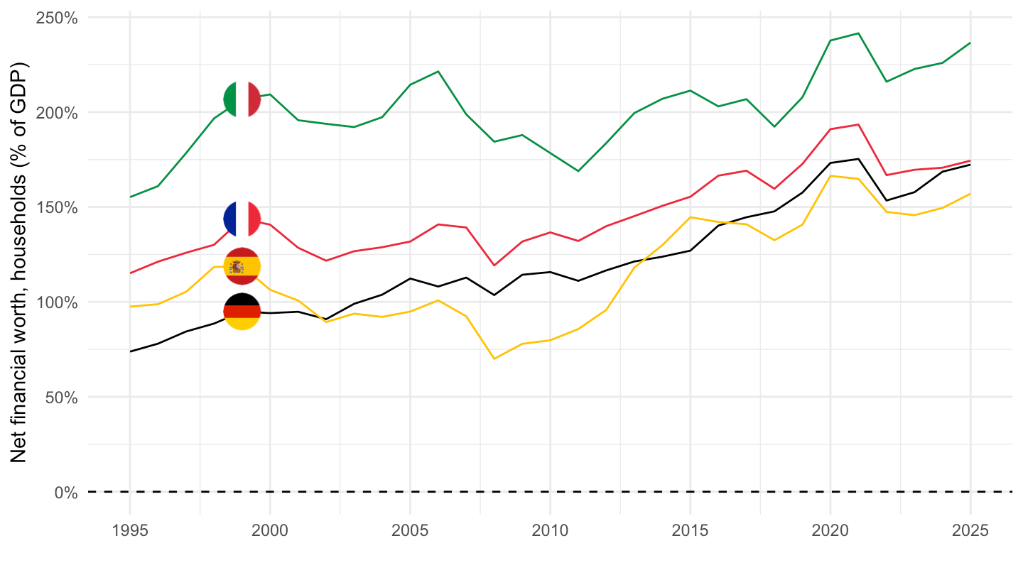

na_item

load_data("eurostat/na_item.RData")
nasa_10_f_bs %>%
  
  group_by(na_item, Na_item) %>%
  summarise(Nobs = n()) %>%
  arrange(-Nobs) %>%
  {if (is_html_output()) datatable(., filter = 'top', rownames = F) else .}

Financial Net Worth - BF90

Table

nasa_10_f_bs %>%
  filter(geo %in% c("FR", "DE"),
         time == "2019", 
         co_nco == "CO",
         na_item == "BF90",
         unit == "PC_GDP") %>%
  
  
  mutate(Geo = ifelse(geo == "DE", "Germany", Geo)) %>%
  mutate(Geo = gsub(" ", "-", str_to_lower(Geo)),
         Geo = paste0('<img src="../../icon/flag/vsmall/', Geo, '.png" alt="Flag">')) %>%
  select(Geo, sector, Sector, values) %>%
  spread(Geo, values) %>%
  {if (is_html_output()) datatable(., filter = 'top', rownames = F, escape = F) else .}

Table

nasa_10_f_bs %>%
  filter(geo %in% c("FR", "DE"),
         sector %in% c("S1", "S11", "S12", "S13", "S14_S15", "S2"),
         time == "2019", 
         co_nco == "CO",
         na_item == "BF90",
         unit == "PC_GDP") %>%
  
  
  mutate(Geo = ifelse(geo == "DE", "Germany", Geo)) %>%
  mutate(Geo = gsub(" ", "-", str_to_lower(Geo)),
         Geo = paste0('<img src="../../icon/flag/vsmall/', Geo, '.png" alt="Flag">')) %>%
  mutate(icon = paste0('<img src="../../icon/sector/vsmall/', sector, '.png" alt="All">')) %>%
  select(icon, Geo, sector, Sector, values) %>%
  spread(Geo, values) %>%
  {if (is_html_output()) datatable(., filter = 'top', rownames = F, escape = F) else .}

Graphs

nasa_10_f_bs %>%
  filter(geo %in% c("FR", "DE"),
         sector %in% c("S11", "S12", "S13", "S14_S15"),
         co_nco == "CO",
         na_item == "BF90",
         unit == "PC_GDP") %>%
  
  mutate(Geo = ifelse(geo == "DE", "Germany", Geo)) %>%
  
  year_to_date %>%
  mutate(values = values/100) %>%
  ggplot(.) + geom_line(aes(x = date, y = values, color = Geo, linetype = Sector)) + 
  theme_minimal() + xlab("") + ylab("% du PIB") +
  scale_x_date(breaks = seq(1960, 2100, 5) %>% paste0("-01-01") %>% as.Date,
               labels = date_format("%Y")) +
  add_flags +
  geom_image(data = tibble(date = rep(as.Date("2020-01-01"), 6),
                           value = c(1.6, 0.1, -0.2, -0.5, -0.75, -.95),
                           image = c("../../icon/sector/vsmall/S14_S15.png",
                                     "../../icon/sector/vsmall/S12.png",
                                     "../../icon/sector/vsmall/S13.png",
                                     "../../icon/sector/vsmall/S11.png",
                                     "../../icon/sector/vsmall/S13.png",
                                     "../../icon/sector/vsmall/S11.png")),
             aes(x = date, y = value, image = image), asp = 1.5) +
  scale_color_manual(values = c("#0055a4", "#000000")) +
  scale_y_continuous(breaks = 0.01*seq(-200, 200, 20),
                     labels = percent_format()) +
  theme(legend.position = "none")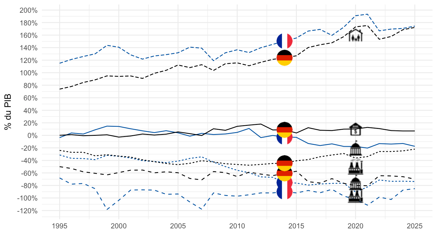

2018, France, Germany, Italy, United Kingdom

All Items

nasa_10_f_bs %>%
  filter(geo %in% c("FR", "DE", "IT", "UK"),
         time == "2019", 
         sector == "S1",
         co_nco == "CO",
         finpos == "ASS",
         unit == "PC_GDP") %>%
  
  
  mutate(Geo = ifelse(geo == "DE", "Germany", Geo)) %>%
  mutate(Geo = gsub(" ", "-", str_to_lower(Geo)),
         Geo = paste0('<img src="../../icon/flag/vsmall/', Geo, '.png" alt="Flag">')) %>%
  select(Geo, na_item, Na_item, values) %>%
  spread(Geo, values) %>%
  {if (is_html_output()) datatable(., filter = 'top', rownames = F, escape = F) else .}

Non-financial corporations

nasa_10_f_bs %>%
  filter(geo %in% c("FR", "DE", "IT", "UK"),
         time == "2019", 
         sector == "S11",
         co_nco == "CO",
         finpos == "ASS",
         unit == "PC_GDP") %>%
  
  
  mutate(Geo = ifelse(geo == "DE", "Germany", Geo)) %>%
  mutate(Geo = gsub(" ", "-", str_to_lower(Geo)),
         Geo = paste0('<img src="../../icon/flag/vsmall/', Geo, '.png" alt="Flag">')) %>%
  select(Geo, na_item, Na_item, values) %>%
  spread(Geo, values) %>%
  {if (is_html_output()) datatable(., filter = 'top', rownames = F, escape = F) else .}

Financial corporations

nasa_10_f_bs %>%
  filter(geo %in% c("FR", "DE", "IT", "UK"),
         time == "2019", 
         sector == "S12",
         co_nco == "CO",
         finpos == "ASS",
         unit == "PC_GDP") %>%
  
  
  mutate(Geo = ifelse(geo == "DE", "Germany", Geo)) %>%
  mutate(Geo = gsub(" ", "-", str_to_lower(Geo)),
         Geo = paste0('<img src="../../icon/flag/vsmall/', Geo, '.png" alt="Flag">')) %>%
  select(Geo, na_item, Na_item, values) %>%
  spread(Geo, values) %>%
  {if (is_html_output()) datatable(., filter = 'top', rownames = F, escape = F) else .}

General government

nasa_10_f_bs %>%
  filter(geo %in% c("FR", "DE", "IT", "UK"),
         time == "2019", 
         sector == "S13",
         co_nco == "CO",
         finpos == "ASS",
         unit == "PC_GDP") %>%
  
  
  mutate(Geo = ifelse(geo == "DE", "Germany", Geo)) %>%
  mutate(Geo = gsub(" ", "-", str_to_lower(Geo)),
         Geo = paste0('<img src="../../icon/flag/vsmall/', Geo, '.png" alt="Flag">')) %>%
  select(Geo, na_item, Na_item, values) %>%
  spread(Geo, values) %>%
  {if (is_html_output()) datatable(., filter = 'top', rownames = F, escape = F) else .}

Households

nasa_10_f_bs %>%
  filter(geo %in% c("FR", "DE", "IT", "UK"),
         time == "2019", 
         sector == "S14_S15",
         co_nco == "CO",
         finpos == "ASS",
         unit == "PC_GDP") %>%
  
  
  mutate(Geo = ifelse(geo == "DE", "Germany", Geo)) %>%
  mutate(Geo = gsub(" ", "-", str_to_lower(Geo)),
         Geo = paste0('<img src="../../icon/flag/vsmall/', Geo, '.png" alt="Flag">')) %>%
  select(Geo, na_item, Na_item, values) %>%
  spread(Geo, values) %>%
  {if (is_html_output()) datatable(., filter = 'top', rownames = F, escape = F) else .}

Rest of the World

nasa_10_f_bs %>%
  filter(geo %in% c("FR", "DE", "IT", "UK"),
         time == "2019", 
         sector == "S2",
         co_nco == "CO",
         finpos == "ASS",
         unit == "PC_GDP") %>%
  
  
  mutate(Geo = ifelse(geo == "DE", "Germany", Geo)) %>%
  mutate(Geo = gsub(" ", "-", str_to_lower(Geo)),
         Geo = paste0('<img src="../../icon/flag/vsmall/', Geo, '.png" alt="Flag">')) %>%
  select(Geo, na_item, Na_item, values) %>%
  spread(Geo, values) %>%
  {if (is_html_output()) datatable(., filter = 'top', rownames = F, escape = F) else .}