| LAST_DOWNLOAD |
|---|
| 2026-07-25 |
Debt service ratios for the private non-financial sector - DSR
Data - BIS
Info
LAST_DOWNLOAD
LAST_COMPILE
| LAST_COMPILE |
|---|
| 2026-07-26 |
Last
| date | Nobs |
|---|---|
| 2025-12-31 | 66 |
Info
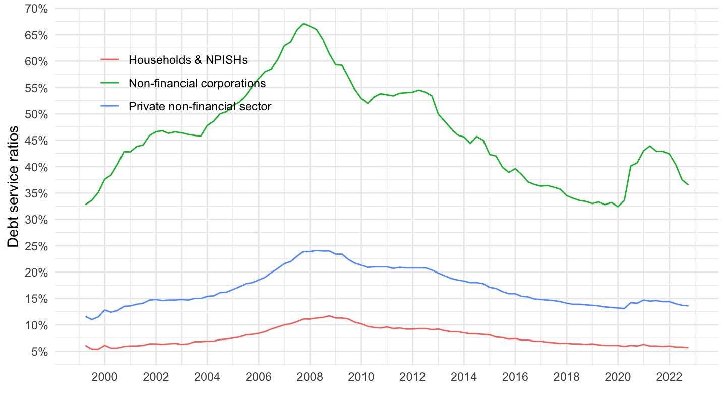
The DSR is defined as the ratio of interest payments plus amortisations to income. As such, the DSR provides a flow-to- flow comparison - the flow of debt service payments divided by the flow of income. More information at https://www.bis.org/publ/qtrpdf/r_qt1509h.htm.
“The DSR is a measure of the proportion of interest payments and mandatory repayments of principals relative to income for the private non-financial sector as a whole and can be interpreted as capturing incipient liquidity constraints of private sector borrowers…. The DSR captures the burden that debt imposes on borrowers more accurately [than other indicators].”
iso3c, iso2c, Borrowers’ country
Code
DSR %>%
  arrange(iso3c, date) %>%
  group_by(iso3c, iso2c, `Borrowers' country`) %>%
  summarise(Nobs = n(),
            start = first(date),
            end = last(date)) %>%
  arrange(-Nobs) %>%
  mutate(Flag = gsub(" ", "-", str_to_lower(`Borrowers' country`)),
         Flag = paste0('<img src="../../icon/flag/vsmall/', Flag, '.png" alt="Flag">')) %>%
  select(Flag, everything()) %>%
  {if (is_html_output()) datatable(., filter = 'top', rownames = F, escape = F) else .}
DSR_BORROWERS, Borrowers
Code
DSR %>%
  group_by(DSR_BORROWERS, Borrowers) %>%
  summarise(Nobs = n()) %>%
  arrange(-Nobs) %>%
print_table_conditional()| DSR_BORROWERS | Borrowers | Nobs |
|---|---|---|
| P | Private non-financial sector | 3444 |
| H | Households & NPISHs | 1836 |
| N | Non-financial corporations | 1836 |
date
Code
DSR %>%
  group_by(date) %>%
  summarise(Nobs = n()) %>%
  arrange(desc(date)) %>%
  print_table_conditional()
Non-financial corporations
Table
Code
DSR %>%
  filter(DSR_BORROWERS == "N") %>%
  group_by(iso2c, `Borrowers' country`) %>%
  summarise(Nobs = n(),
            `2008Q1` = value[date == as.Date("2008-03-31")],
            `2020Q4` = value[date == as.Date("2020-12-31")]) %>%
  mutate(`growth` = `2020Q4`/`2008Q1` - 1) %>%
  arrange(growth) %>%
  mutate(Flag = gsub(" ", "-", str_to_lower(`Borrowers' country`)),
         Flag = paste0('<img src="../../icon/flag/vsmall/', Flag, '.png" alt="Flag">')) %>%
  select(Flag, everything()) %>%
  {if (is_html_output()) datatable(., filter = 'top', rownames = F, escape = F) else .}
Australia, United States, United Kingdom
Code
DSR %>%
  filter(iso2c %in% c("GB", "AU", "US"),
         DSR_BORROWERS == "N") %>%
  left_join(colors, by = c("Borrowers' country" = "country")) %>%
  ggplot(.) +
  geom_line(aes(x = date, y = value/100, color = color)) +
  theme_minimal() + xlab("") + ylab("Debt service ratios - Non-financial corporations") +
  scale_color_identity() + add_flags +
  scale_x_date(breaks = seq(1940, 2100, 2) %>% paste0("-01-01") %>% as.Date,
               labels = date_format("%Y")) +
  scale_y_continuous(breaks = 0.01*seq(-5, 100, 5),
                labels = percent_format(accuracy = 1)) +
  theme(legend.position = c(0.5, 0.9),
        legend.title = element_blank())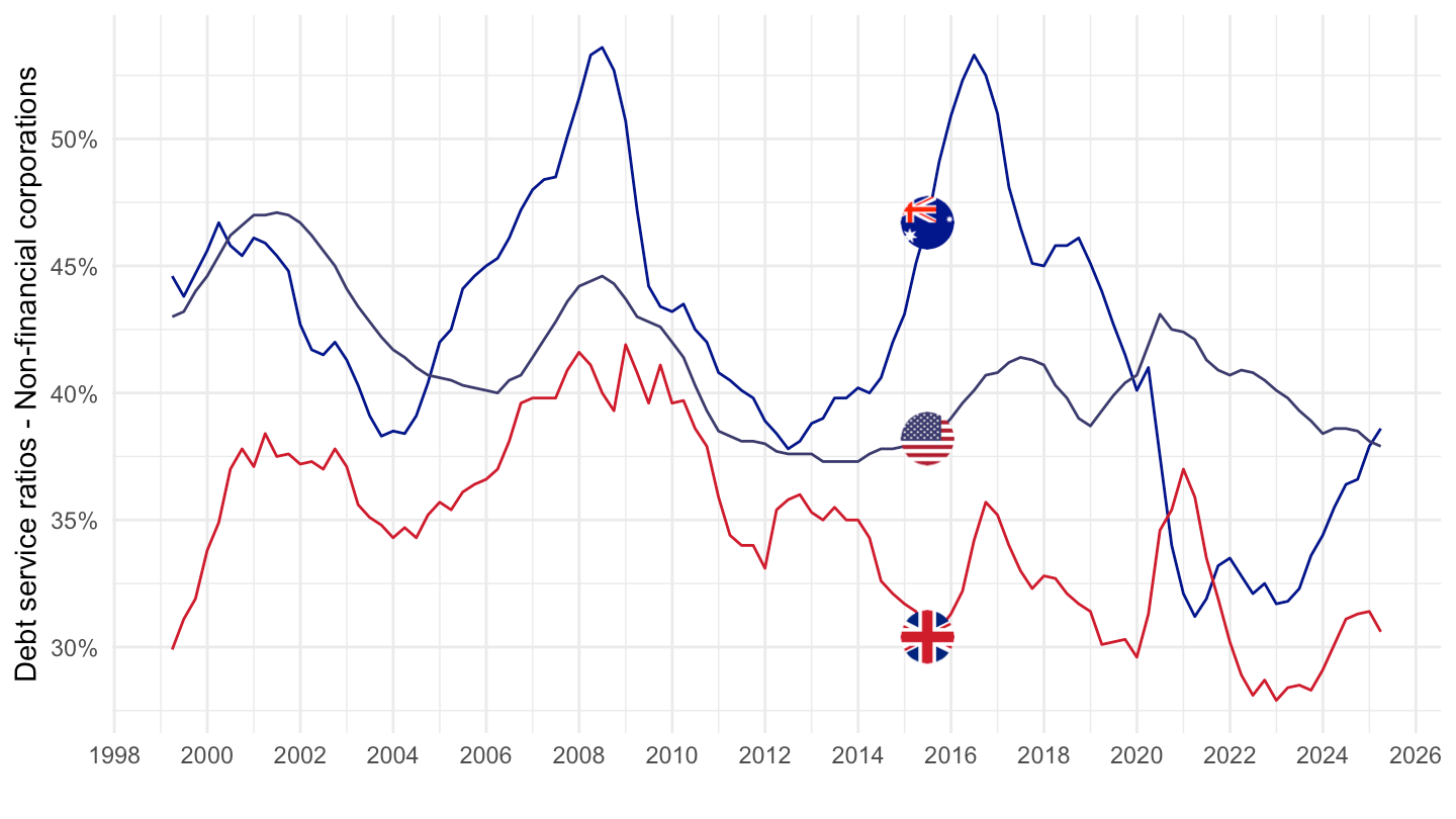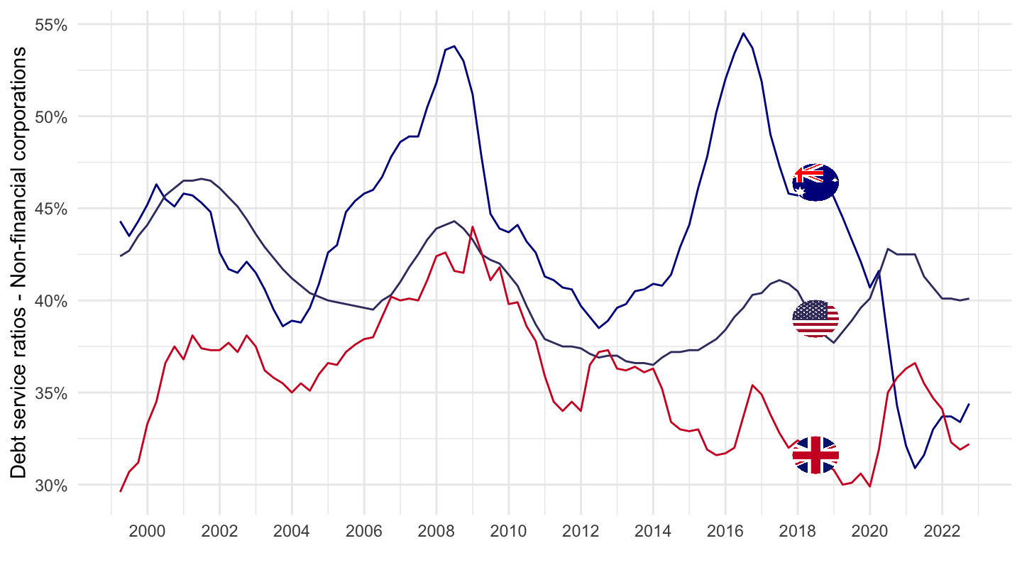
Denmark, Spain, United Kingdom
Code
DSR %>%
  filter(iso2c %in% c("GB", "ES", "DK"),
         DSR_BORROWERS == "N") %>%
  left_join(colors, by = c("Borrowers' country" = "country")) %>%
  ggplot(.) +
  geom_line(aes(x = date, y = value/100, color = color)) +
  theme_minimal() + xlab("") + ylab("Debt service ratios - Non-financial corporations") +
  scale_color_identity() + add_flags +
  scale_x_date(breaks = seq(1940, 2100, 2) %>% paste0("-01-01") %>% as.Date,
               labels = date_format("%Y")) +
  scale_y_continuous(breaks = 0.01*seq(-5, 100, 5),
                labels = percent_format(accuracy = 1)) +
  theme(legend.position = c(0.5, 0.9),
        legend.title = element_blank())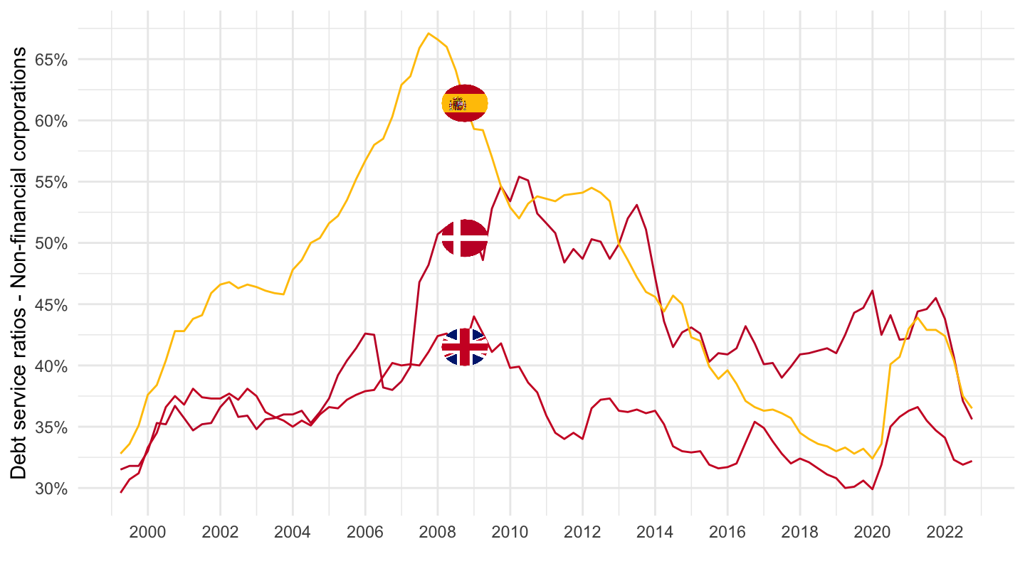
France, Spain, Italy
Code
DSR %>%
  filter(iso2c %in% c("ES", "IT", "FR"),
         DSR_BORROWERS == "N") %>%
  left_join(colors, by = c("Borrowers' country" = "country")) %>%
  ggplot(.) +
  geom_line(aes(x = date, y = value/100, color = color)) +
  theme_minimal() + xlab("") + ylab("Debt service ratios - Non-financial corporations") +
  scale_color_identity() + add_flags +
  scale_x_date(breaks = seq(1940, 2100, 2) %>% paste0("-01-01") %>% as.Date,
               labels = date_format("%Y")) +
  scale_y_continuous(breaks = 0.01*seq(-5, 100, 5),
                labels = percent_format(accuracy = 1)) +
  theme(legend.position = c(0.5, 0.9),
        legend.title = element_blank())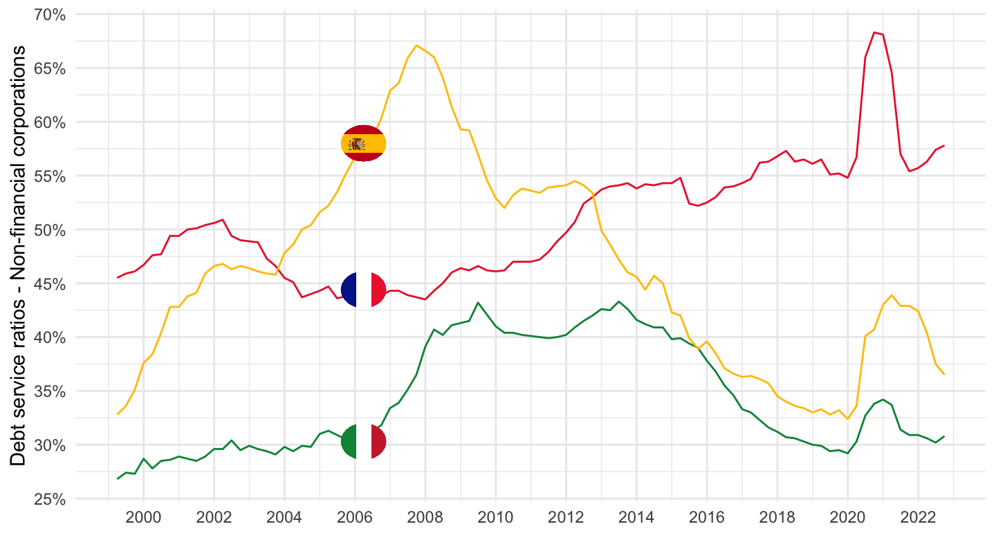
Italy, Portugal, Spain
Code
DSR %>%
  filter(iso2c %in% c("ES", "IT", "PT"),
         DSR_BORROWERS == "N") %>%
  left_join(colors, by = c("Borrowers' country" = "country")) %>%
  ggplot(.) +
  geom_line(aes(x = date, y = value/100, color = color)) +
  theme_minimal() + xlab("") + ylab("Debt service ratios - Non-financial corporations") +
  scale_color_identity() + add_flags +
  scale_x_date(breaks = seq(1940, 2100, 2) %>% paste0("-01-01") %>% as.Date,
               labels = date_format("%Y")) +
  scale_y_continuous(breaks = 0.01*seq(-5, 100, 5),
                labels = percent_format(accuracy = 1)) +
  theme(legend.position = c(0.5, 0.9),
        legend.title = element_blank())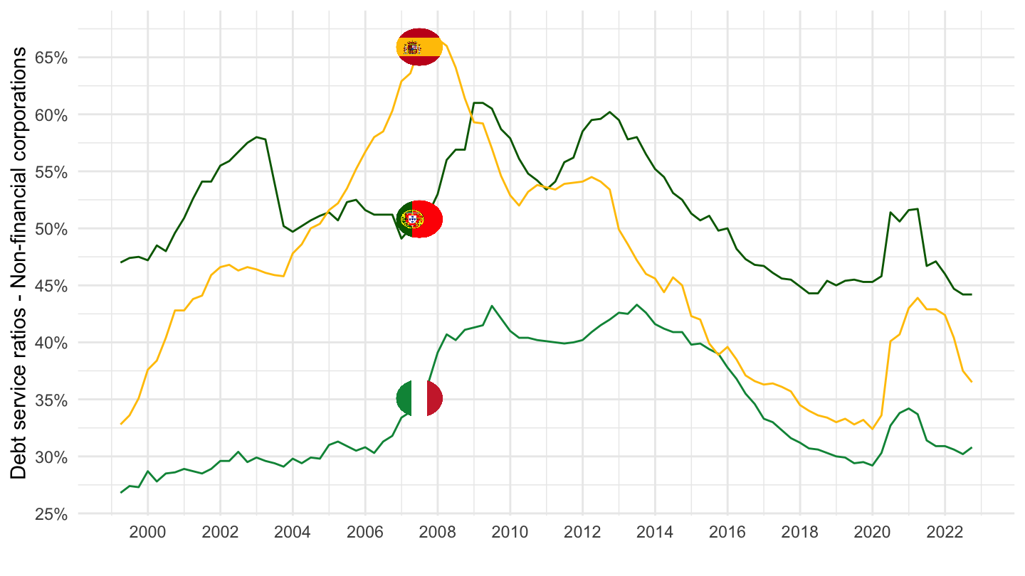
France, Germany, United States
Code
DSR %>%
  filter(iso2c %in% c("US", "FR", "DE"),
         DSR_BORROWERS == "N") %>%
  left_join(colors, by = c("Borrowers' country" = "country")) %>%
  ggplot(.) +
  geom_line(aes(x = date, y = value/100, color = color)) +
  theme_minimal() + xlab("") + ylab("Debt service ratios - Non-financial corporations") +
  scale_color_identity() + add_flags +
  scale_x_date(breaks = seq(1940, 2100, 2) %>% paste0("-01-01") %>% as.Date,
               labels = date_format("%Y")) +
  scale_y_continuous(breaks = 0.01*seq(-5, 100, 5),
                labels = percent_format(accuracy = 1)) +
  theme(legend.position = c(0.5, 0.9),
        legend.title = element_blank())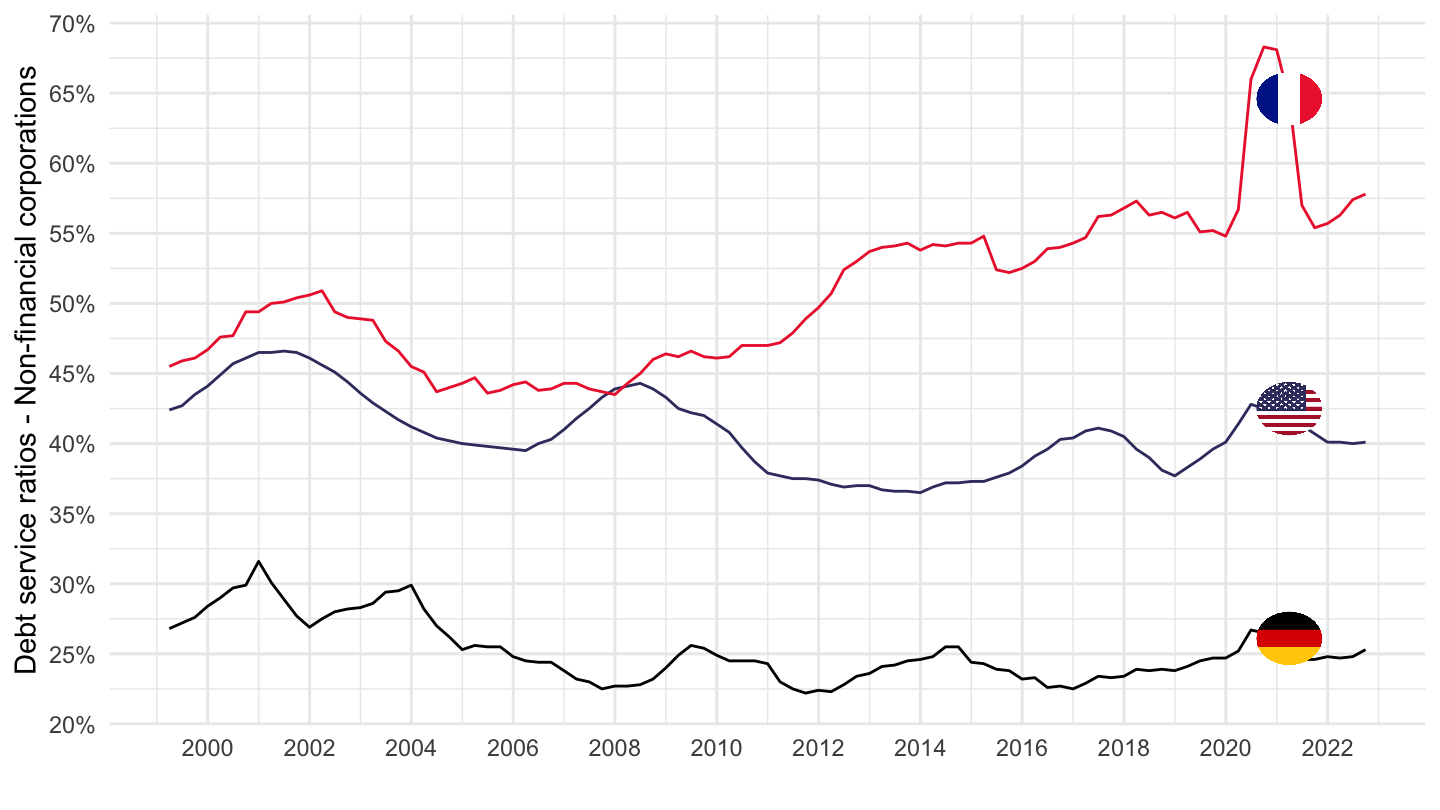
Sweden, France, Canada
Code
DSR %>%
  filter(iso2c %in% c("CA", "SE", "FR"),
         DSR_BORROWERS == "N") %>%
  left_join(colors, by = c("Borrowers' country" = "country")) %>%
  ggplot(.) +
  geom_line(aes(x = date, y = value/100, color = color)) +
  theme_minimal() + xlab("") + ylab("Debt service ratios - Non-financial corporations") +
  scale_color_identity() + add_flags +
  scale_x_date(breaks = seq(1940, 2100, 2) %>% paste0("-01-01") %>% as.Date,
               labels = date_format("%Y")) +
  scale_y_continuous(breaks = 0.01*seq(-5, 100, 5),
                labels = percent_format(accuracy = 1)) +
  theme(legend.position = c(0.5, 0.9),
        legend.title = element_blank())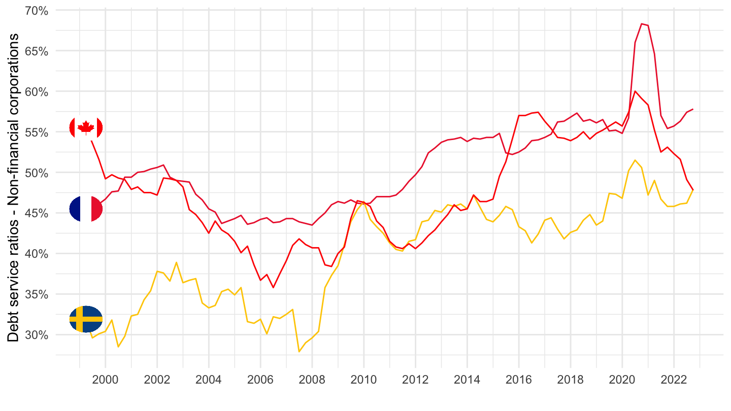
Private non-financial sector
Table
Code
DSR %>%
  filter(DSR_BORROWERS == "P") %>%
  group_by(iso2c, `Borrowers' country`) %>%
  summarise(Nobs = n(),
            `2008Q1` = value[date == as.Date("2008-03-31")],
            `2020Q4` = value[date == as.Date("2020-12-31")]) %>%
  mutate(`growth` = `2020Q4`/`2008Q1` - 1) %>%
  arrange(growth) %>%
  mutate(Flag = gsub(" ", "-", str_to_lower(`Borrowers' country`)),
         Flag = paste0('<img src="../../icon/flag/vsmall/', Flag, '.png" alt="Flag">')) %>%
  select(Flag, everything()) %>%
  {if (is_html_output()) datatable(., filter = 'top', rownames = F, escape = F) else .}
France, Germany, United States
Code
DSR %>%
  filter(iso2c %in% c("FR", "DE", "US"),
         DSR_BORROWERS == "P") %>%
  left_join(colors, by = c("Borrowers' country" = "country")) %>%
  ggplot(.) +
  geom_line(aes(x = date, y = value/100, color = color)) +
  theme_minimal() + xlab("") + ylab("Debt service ratios - Private non-financial sector") +
  scale_color_identity() + add_flags +
  scale_x_date(breaks = seq(1940, 2100, 2) %>% paste0("-01-01") %>% as.Date,
               labels = date_format("%Y")) +
  scale_y_continuous(breaks = 0.01*seq(-5, 30, 1),
                labels = percent_format(accuracy = 1)) +
  theme(legend.position = c(0.8, 0.65),
        legend.title = element_blank())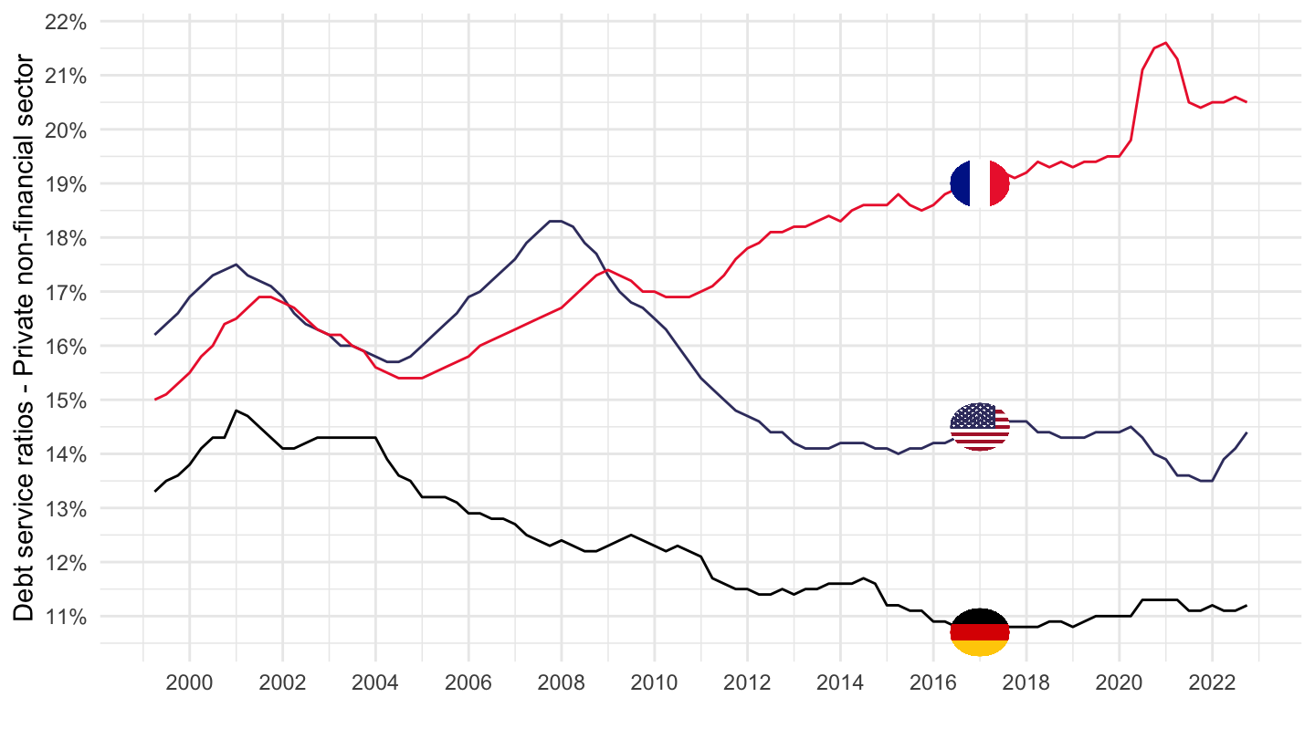
France, Germany, United States
All
Code
DSR %>%
  filter(iso2c %in% c("FR", "DE", "US", "FI"),
         DSR_BORROWERS == "P") %>%
  left_join(colors, by = c("Borrowers' country" = "country")) %>%
  ggplot(.) +
  geom_line(aes(x = date, y = value/100, color = color)) +
  theme_minimal() + xlab("") + ylab("Debt service ratios - Private non-financial sector") +
  scale_color_identity() + add_flags +
  scale_x_date(breaks = seq(1940, 2100, 2) %>% paste0("-01-01") %>% as.Date,
               labels = date_format("%Y")) +
  scale_y_continuous(breaks = 0.01*seq(-5, 30, 1),
                labels = percent_format(accuracy = 1)) +
  theme(legend.position = c(0.8, 0.65),
        legend.title = element_blank())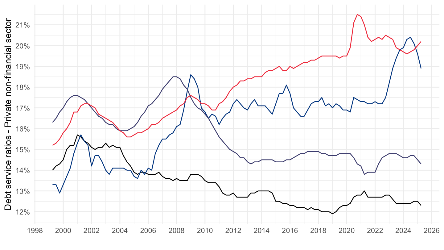
France, Spain, Italy
Code
DSR %>%
  filter(iso2c %in% c("FR", "ES", "IT"),
         DSR_BORROWERS == "P") %>%
  left_join(colors, by = c("Borrowers' country" = "country")) %>%
  ggplot(.) +
  geom_line(aes(x = date, y = value/100, color = color)) +
  theme_minimal() + xlab("") + ylab("Debt service ratios - Private non-financial sector") +
  scale_color_identity() + add_flags +
  scale_x_date(breaks = seq(1940, 2100, 2) %>% paste0("-01-01") %>% as.Date,
               labels = date_format("%Y")) +
  scale_y_continuous(breaks = 0.01*seq(-5, 100, 1),
                labels = percent_format(accuracy = 1)) +
  theme(legend.position = c(0.8, 0.9),
        legend.title = element_blank())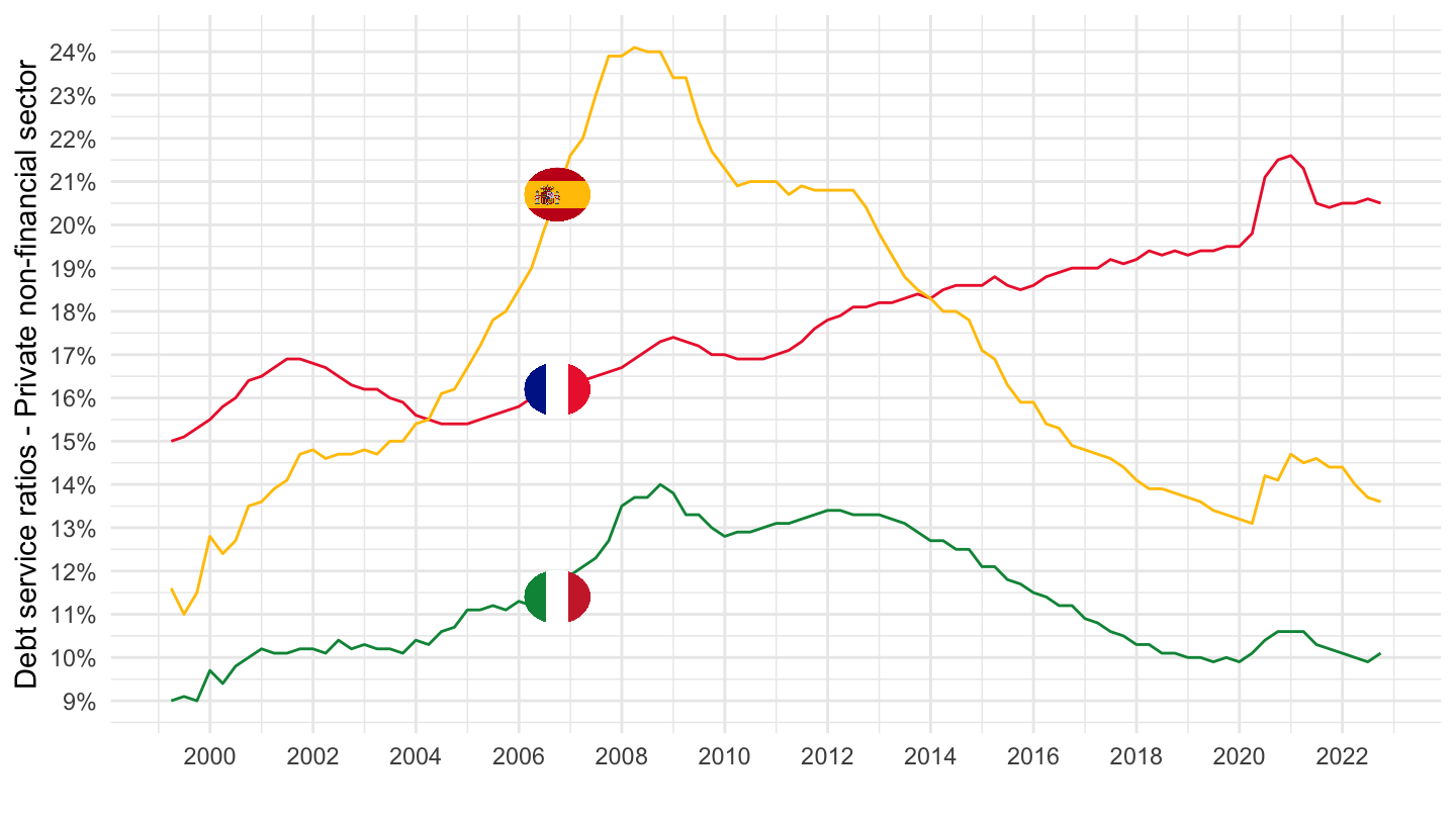
Households & NPISHs
Table
Code
DSR %>%
  filter(DSR_BORROWERS == "H") %>%
  group_by(iso2c, `Borrowers' country`) %>%
  summarise(Nobs = n(),
            `2008Q1` = value[date == as.Date("2008-03-31")],
            `2020Q4` = value[date == as.Date("2020-12-31")]) %>%
  mutate(`growth` = `2020Q4`/`2008Q1` - 1) %>%
  arrange(growth) %>%
  mutate(Flag = gsub(" ", "-", str_to_lower(`Borrowers' country`)),
         Flag = paste0('<img src="../../icon/flag/vsmall/', Flag, '.png" alt="Flag">')) %>%
  select(Flag, everything()) %>%
  {if (is_html_output()) datatable(., filter = 'top', rownames = F, escape = F) else .}
France, Germany, United States
Code
DSR %>%
  filter(iso2c %in% c("FR", "DE", "US"),
         DSR_BORROWERS == "H") %>%
  left_join(colors, by = c("Borrowers' country" = "country")) %>%
  ggplot(.) +
  geom_line(aes(x = date, y = value/100, color = color)) +
  theme_minimal() + xlab("") + ylab("Debt service ratios - Households & NPISHs") +
  scale_color_identity() + add_flags +
  scale_x_date(breaks = seq(1940, 2100, 2) %>% paste0("-01-01") %>% as.Date,
               labels = date_format("%Y")) +
  scale_y_continuous(breaks = 0.01*seq(-5, 100, 1),
                labels = percent_format(accuracy = 1)) +
  theme(legend.position = c(0.8, 0.9),
        legend.title = element_blank())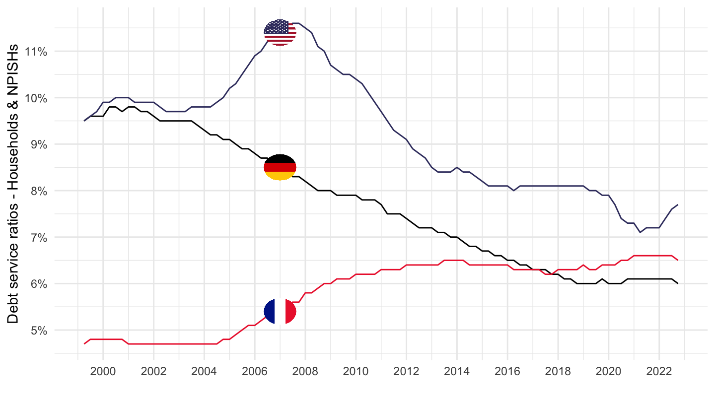
France, Spain, Italy
Code
DSR %>%
  filter(iso2c %in% c("FR", "ES", "IT"),
         DSR_BORROWERS == "H") %>%
  left_join(colors, by = c("Borrowers' country" = "country")) %>%
  ggplot(.) +
  geom_line(aes(x = date, y = value/100, color = color)) +
  theme_minimal() + xlab("") + ylab("Debt service ratios - Households & NPISHs") +
  scale_color_identity() + add_flags +
  scale_x_date(breaks = seq(1940, 2100, 2) %>% paste0("-01-01") %>% as.Date,
               labels = date_format("%Y")) +
  scale_y_continuous(breaks = 0.01*seq(-5, 100, 1),
                labels = percent_format(accuracy = 1)) +
  theme(legend.position = c(0.8, 0.9),
        legend.title = element_blank())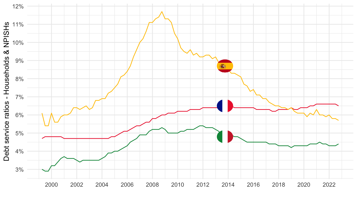
Sweden, France, Canada
Code
DSR %>%
  filter(iso2c %in% c("CA", "SE", "FR"),
         DSR_BORROWERS == "H") %>%
  left_join(colors, by = c("Borrowers' country" = "country")) %>%
  ggplot(.) +
  geom_line(aes(x = date, y = value/100, color = color)) +
  theme_minimal() + xlab("") + ylab("Debt service ratios - Households & NPISHs") +
  scale_color_identity() + add_flags +
  scale_x_date(breaks = seq(1940, 2100, 2) %>% paste0("-01-01") %>% as.Date,
               labels = date_format("%Y")) +
  scale_y_continuous(breaks = 0.01*seq(-5, 100, 1),
                labels = percent_format(accuracy = 1)) +
  theme(legend.position = c(0.5, 0.9),
        legend.title = element_blank())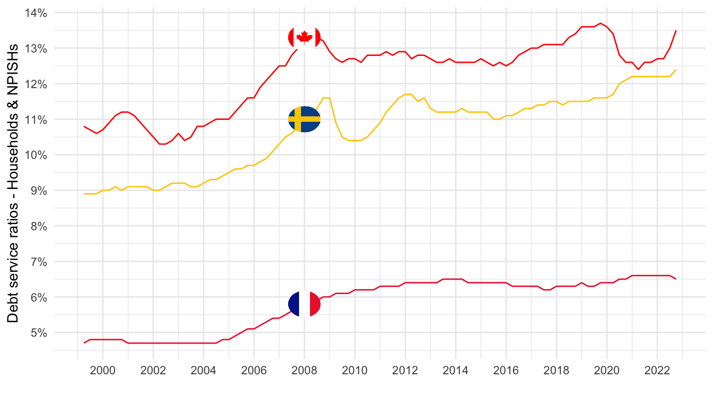
Sectors
Germany
Code
DSR %>%
  filter(iso3c %in% c("DEU")) %>%
  ggplot(.) + theme_minimal() + xlab("") + ylab("Debt service ratios") +
  geom_line(aes(x = date, y = value/100, color = Borrowers)) +
  scale_x_date(breaks = seq(1940, 2100, 2) %>% paste0("-01-01") %>% as.Date,
               labels = date_format("%Y")) +
  scale_y_continuous(breaks = 0.01*seq(0, 100, 2),
                labels = percent_format(accuracy = 1)) +

  theme(legend.position = c(0.2, 0.8),
        legend.title = element_blank())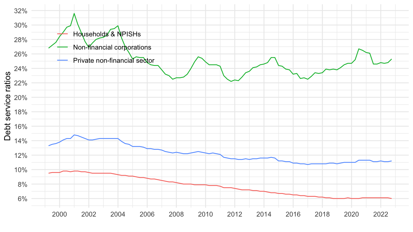
France
Code
DSR %>%
  filter(iso2c %in% c("FR")) %>%
  ggplot(.) +
  geom_line(aes(x = date, y = value/100, color = Borrowers)) +
  theme_minimal() + xlab("") + ylab("Debt service ratios") +
  scale_x_date(breaks = seq(1940, 2100, 2) %>% paste0("-01-01") %>% as.Date,
               labels = date_format("%Y")) +
  scale_y_continuous(breaks = 0.01*seq(-5, 100, 5),
                labels = percent_format(accuracy = 1)) +
  scale_color_manual(values = viridis(5)[1:4]) +
  theme(legend.position = c(0.8, 0.6),
        legend.title = element_blank())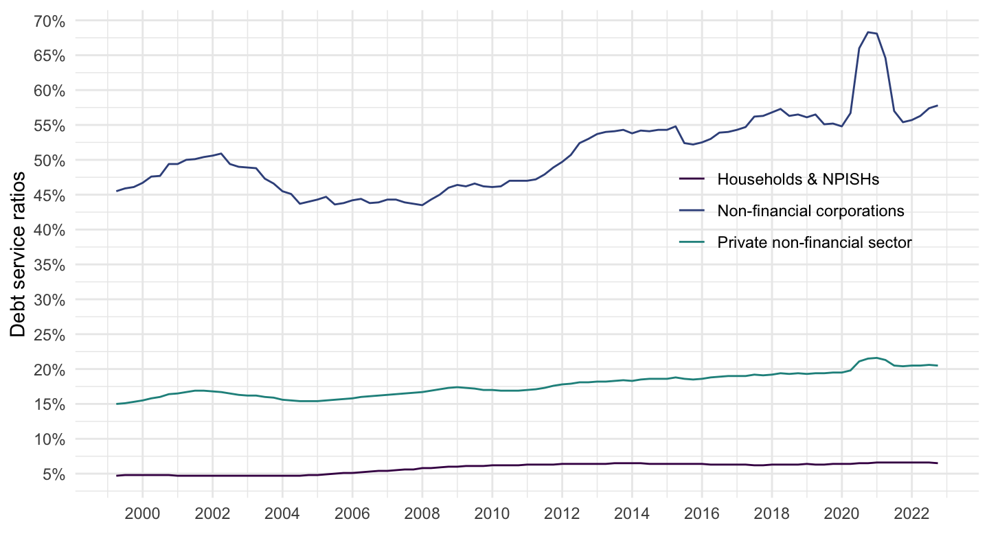
Denmark
Code
DSR %>%
  filter(iso3c %in% c("DNK")) %>%
  ggplot(.) +
  geom_line(aes(x = date, y = value/100, color = Borrowers)) +
  theme_minimal() + xlab("") + ylab("Debt service ratios") +
  scale_x_date(breaks = seq(1940, 2100, 2) %>% paste0("-01-01") %>% as.Date,
               labels = date_format("%Y")) +
  scale_y_continuous(breaks = 0.01*seq(-5, 100, 5),
                labels = percent_format(accuracy = 1)) +

  theme(legend.position = c(0.2, 0.8),
        legend.title = element_blank())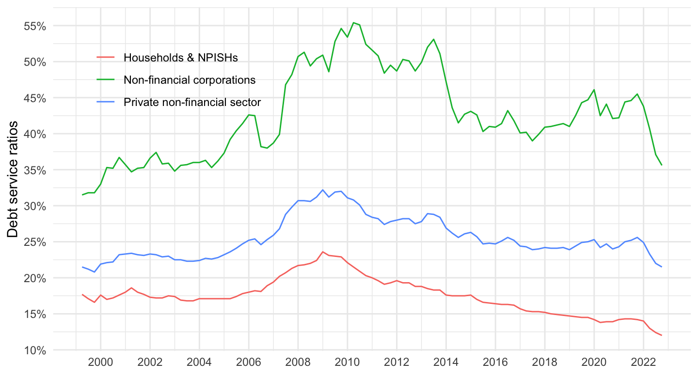
United States
Code
DSR %>%
  filter(iso3c %in% c("USA")) %>%
  ggplot(.) +
  geom_line(aes(x = date, y = value/100, color = Borrowers)) +
  theme_minimal() + xlab("") + ylab("Debt service ratios") +
  scale_x_date(breaks = seq(1940, 2100, 2) %>% paste0("-01-01") %>% as.Date,
               labels = date_format("%Y")) +
  scale_y_continuous(breaks = 0.01*seq(-5, 100, 5),
                labels = percent_format(accuracy = 1)) +

  theme(legend.position = c(0.2, 0.8),
        legend.title = element_blank())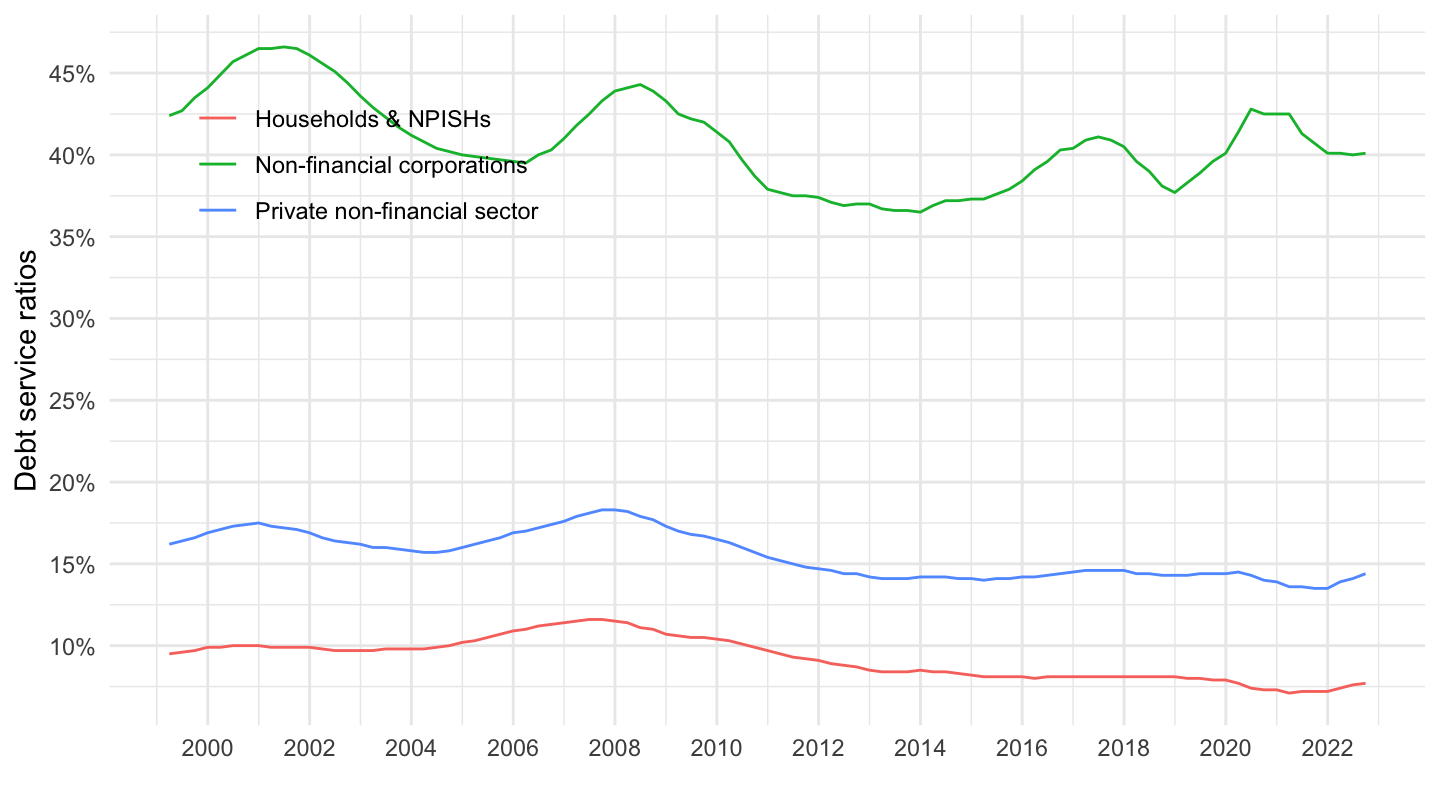
United Kingdom
Code
DSR %>%
  filter(iso3c %in% c("GBR")) %>%
  ggplot(.) + theme_minimal() + xlab("") + ylab("Debt service ratios") +
  geom_line(aes(x = date, y = value/100, color = Borrowers)) +
  scale_x_date(breaks = seq(1940, 2100, 2) %>% paste0("-01-01") %>% as.Date,
               labels = date_format("%Y")) +
  scale_y_continuous(breaks = 0.01*seq(-5, 100, 5),
                labels = percent_format(accuracy = 1)) +
  theme(legend.position = c(0.2, 0.8),
        legend.title = element_blank())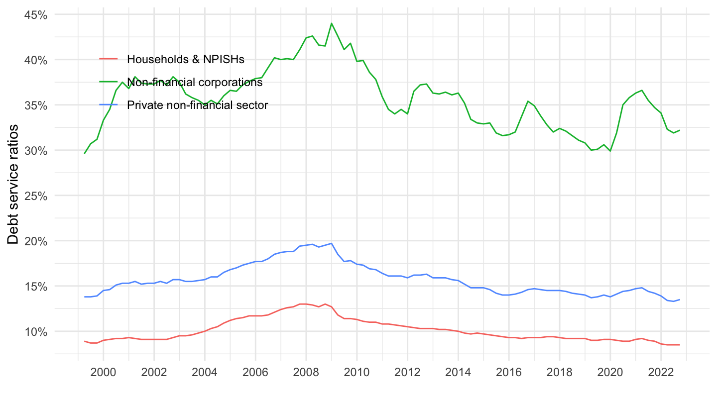
Spain
Code
DSR %>%
  filter(iso3c %in% c("ESP")) %>%
  ggplot(.) + theme_minimal() + xlab("") + ylab("Debt service ratios") +
  geom_line(aes(x = date, y = value/100, color = Borrowers)) +
  scale_x_date(breaks = seq(1940, 2100, 2) %>% paste0("-01-01") %>% as.Date,
               labels = date_format("%Y")) +
  scale_y_continuous(breaks = 0.01*seq(-5, 100, 5),
                labels = percent_format(accuracy = 1)) +

  theme(legend.position = c(0.2, 0.8),
        legend.title = element_blank())