Table 2.1. Personal Income and Its Disposition (A) (Q) - T20100

Name: Table 2.1. Personal Income and Its Disposition (A) (Q)
Creator: François Geerolf
License: https://www.usa.gov/government-works

Data - BEA

Author

François Geerolf

Last observation: Q2 2022 (N = 42) · 2021 (N = 42)

First observation: 1929 (N = 35) · Q1 1947 (N = 38)

Last data update: 25 juil. 2026, 12:36

Last compile: 05 sept. 2026, 22:42

Layout

NIPA Website. html

Comments

Compensation of employees (70%) includes 56% of Wages and salaries:
- Supplements to wages and salaries (14%)
- Supplements include employer contributions (employee pension + insurance + government insurance)
In Wages and salaries = 56.5%:
- 8.9% = Government (acyclical)
- 47.6% = Private (cyclical)
Supplements to wages and salaries (14%) = acyclical.
Dividends are only very mildly cyclical?
Rental income (5% only):
- Net of interest (not like in France?)
- Net of depreciation
Personal income receipts on assets:
- Includes mortgage interest which was not included in rents.
- Proof: Personal interest income and rental income of persons are NEGATIVELY CORRELATED.
Disposable personal/household income:
- 75% in USA.
- Much higher in France?

Disposable personal income / Personal income as a % of GDP

Code

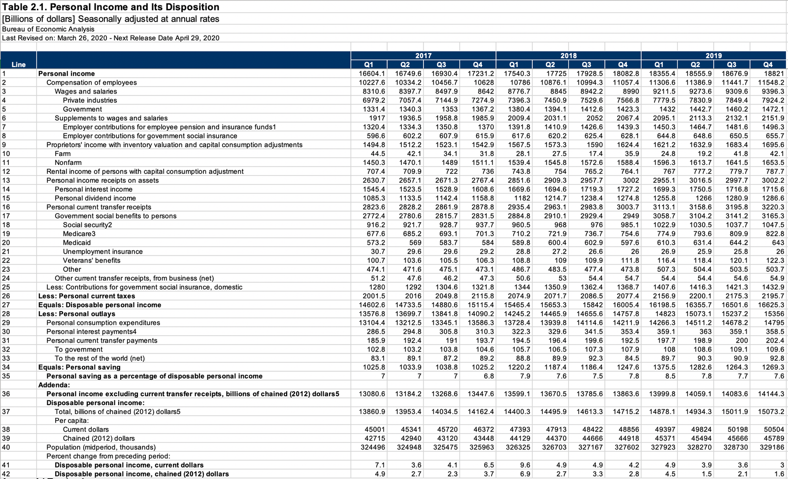
T20100_A |>
  mutate(table = "T20100") |>
  bind_rows(T10105_A |>
              mutate(table = "T10105")) |>
  year_to_date() |>
  arrange(date, LineNumber) |>
  group_by(date) |>
  mutate(value = DataValue/DataValue[LineDescription == "Gross domestic product"]) |>
  filter(LineNumber %in% c(27, 1),
         table == "T20100") |>
  ggplot() + theme_minimal() + 
  geom_line(aes(x = date, y = value, color = LineDescription, linetype = LineDescription)) +
  theme(legend.title = element_blank(),
        legend.position = c(0.3, 0.9)) +
  geom_rect(data = nber_recessions |>
              filter(Peak > as.Date("1929-01-01")), 
            aes(xmin = Peak, xmax = Trough, ymin = -Inf, ymax = +Inf), 
            fill = 'grey', alpha = 0.5) + 
  scale_x_date(breaks = seq(1930, 2100, 5) |> paste0("-01-01") |> as.Date(),
               labels = date_format("%Y")) +
  ylab("% of GDP") + xlab("") +
  scale_color_manual(values = viridis(5)[1:4]) +
  scale_y_continuous(breaks = 0.01*seq(0, 100, 1),
                     labels = scales::percent_format(accuracy = 1))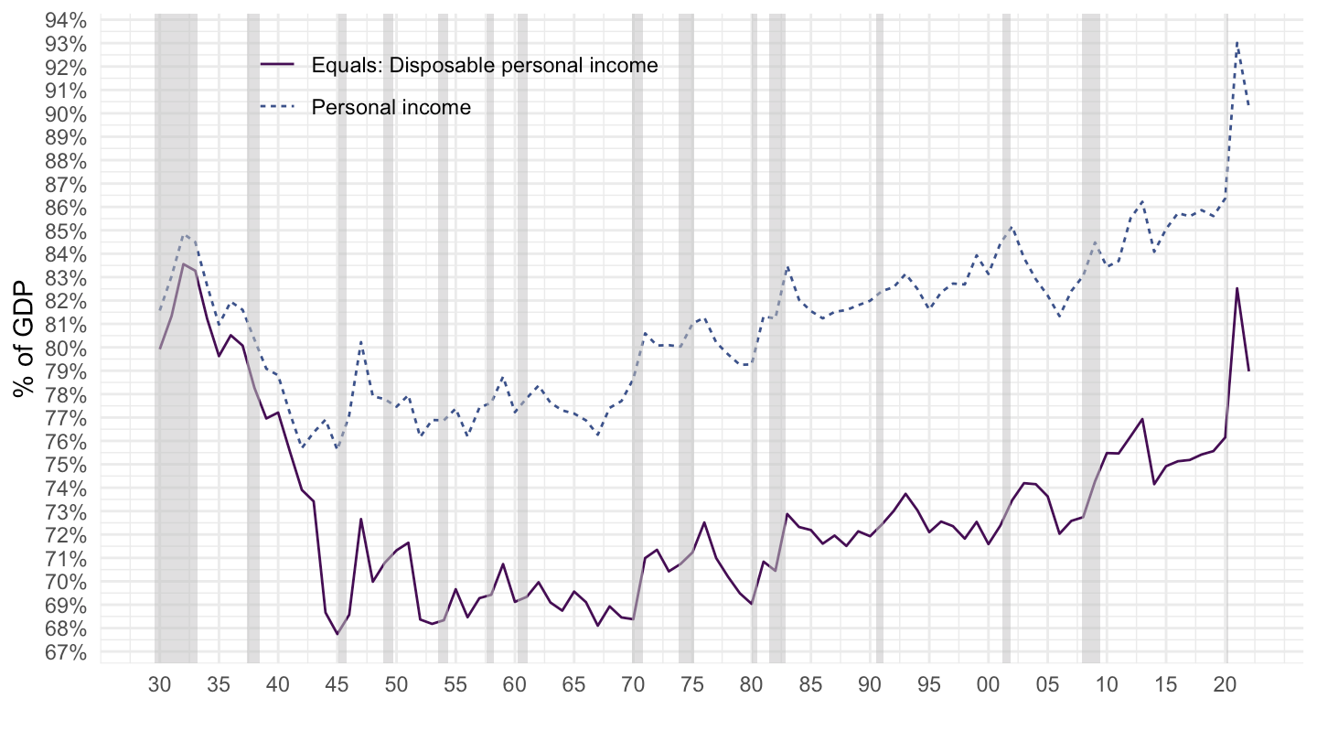

Rental income of persons with capital consumption adjustment

Code

T20100_A |>
  year_to_date() |>
  arrange(date, LineNumber) |>
  group_by(date) |>
  mutate(value = DataValue/DataValue[LineNumber == 27]) |>
  filter(LineNumber %in% c(12, 13, 14, 15)) |>
  ggplot() + theme_minimal() + 
  geom_line(aes(x = date, y = value, color = LineDescription, linetype = LineDescription)) +
  theme(legend.title = element_blank(),
        legend.position = c(0.3, 0.9)) +
  geom_rect(data = nber_recessions |>
              filter(Peak > as.Date("1929-01-01")), 
            aes(xmin = Peak, xmax = Trough, ymin = -Inf, ymax = +Inf), 
            fill = 'grey', alpha = 0.5) + 
  scale_x_date(breaks = seq(1930, 2100, 5) |> paste0("-01-01") |> as.Date(),
               labels = date_format("%Y")) +
  ylab("% of Disposable personal income") + xlab("") +
  scale_color_manual(values = viridis(5)[1:4]) +
  scale_y_continuous(breaks = 0.01*seq(0, 25, 1),
                     labels = scales::percent_format(accuracy = 1))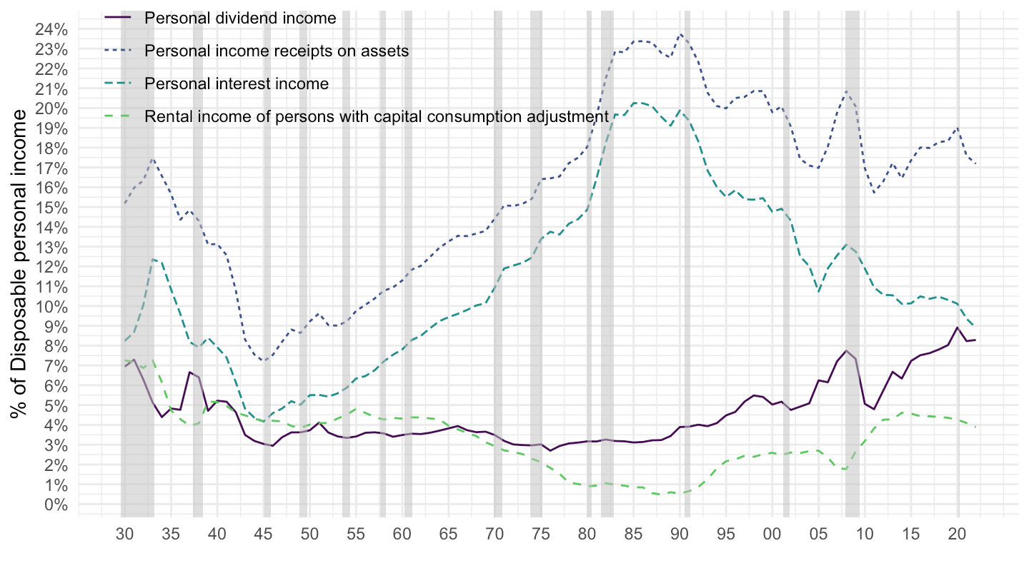

Taxes

Code

T20100_A |>
  year_to_date() |>
  group_by(date) |>
  mutate(value = DataValue/DataValue[LineNumber == 27]) |>
  filter(LineNumber %in% c(26, 6)) |>
  ggplot() + theme_minimal() + 
  geom_line(aes(x = date, y = value, color = LineDescription, linetype = LineDescription)) +
  theme(legend.title = element_blank(),
        legend.position = c(0.75, 0.2)) +
  geom_rect(data = nber_recessions |>
              filter(Peak > as.Date("1928-01-01")), 
            aes(xmin = Peak, xmax = Trough, ymin = 0, ymax = +Inf), 
            fill = 'grey', alpha = 0.5) + 
  scale_x_date(breaks = seq(1925, 2100, 5) |> paste0("-01-01") |> as.Date(),
               labels = date_format("%Y")) +
  ylab("% of Disposable personal income") + xlab("") +
  scale_color_manual(values = viridis(5)[1:4]) +
  scale_y_continuous(breaks = 0.01*seq(0, 90, 2),
                     labels = scales::percent_format(accuracy = 1))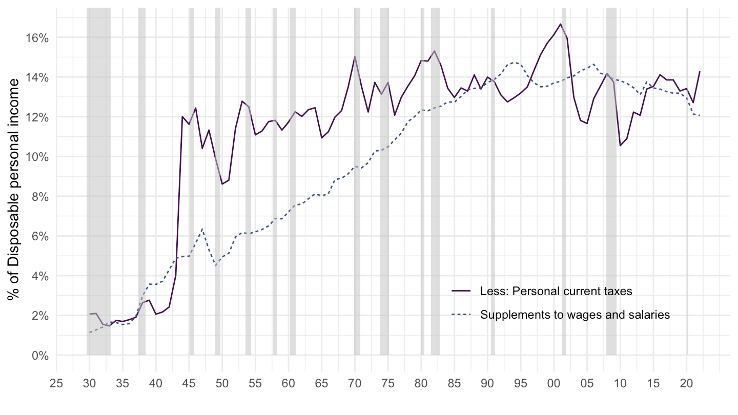

Wages and Salaries / Private VS Government

Code

T20100_A |>
  year_to_date() |>
  group_by(date) |>
  mutate(value = DataValue/DataValue[LineNumber == 27]) |>
  filter(LineNumber %in% c(3, 4, 5)) |>
  ggplot() + theme_minimal() + 
  geom_line(aes(x = date, y = value, color = LineDescription, linetype = LineDescription)) +
  theme(legend.title = element_blank(),
        legend.position = c(0.45, 0.5)) +
  geom_rect(data = nber_recessions |>
              filter(Peak > as.Date("1928-01-01")), 
            aes(xmin = Peak, xmax = Trough, ymin = 0, ymax = +Inf), 
            fill = 'grey', alpha = 0.5) + 
  scale_x_date(breaks = seq(1925, 2100, 5) |> paste0("-01-01") |> as.Date(),
               labels = date_format("%Y")) +
  ylab("% of Disposable personal income") + xlab("") +
  scale_color_manual(values = viridis(5)[1:4]) +
  scale_y_continuous(breaks = 0.01*seq(0, 90, 10),
                     labels = scales::percent_format(accuracy = 1))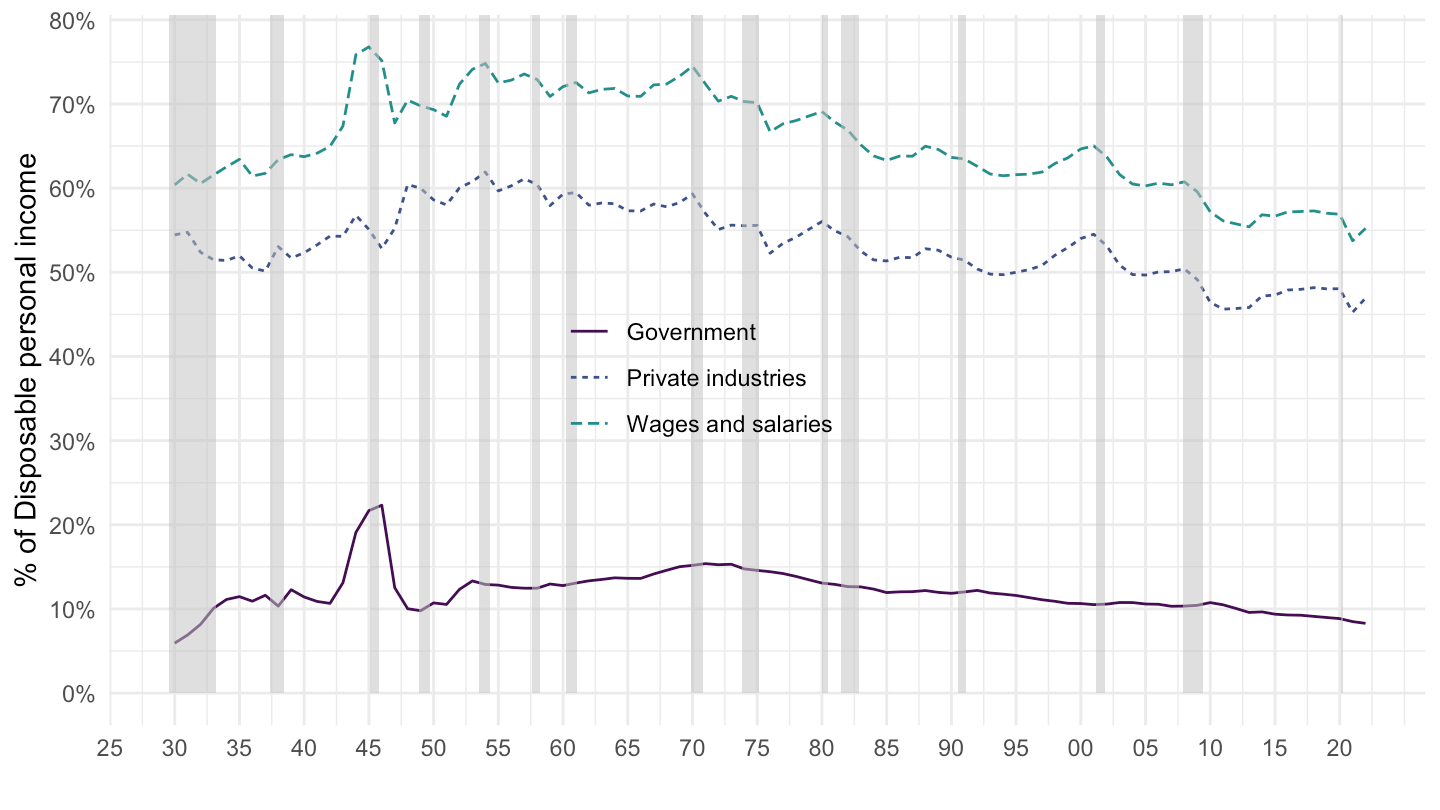

Compensation of Employees

Code

T20100_A |>
  year_to_date() |>
  group_by(date) |>
  mutate(value = DataValue/DataValue[LineNumber == 27]) |>
  filter(LineNumber %in% c(2, 3, 6, 9)) |>
  ggplot() + theme_minimal() + 
  geom_line(aes(x = date, y = value, color = LineDescription, linetype = LineDescription)) +
  theme(legend.title = element_blank(),
        legend.position = c(0.45, 0.5)) +
  geom_rect(data = nber_recessions |>
              filter(Peak > as.Date("1928-01-01")), 
            aes(xmin = Peak, xmax = Trough, ymin = 0, ymax = +Inf), 
            fill = 'grey', alpha = 0.5) + 
  scale_x_date(breaks = seq(1925, 2100, 5) |> paste0("-01-01") |> as.Date(),
               labels = date_format("%Y")) +
  ylab("% of Disposable personal income") + xlab("") +
  scale_color_manual(values = viridis(5)[1:4]) +
  scale_y_continuous(breaks = 0.01*seq(0, 90, 10),
                     labels = scales::percent_format(accuracy = 1))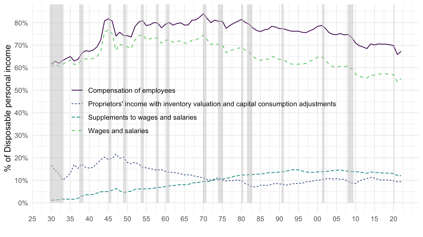

Government

Code

T20100_A |>
  year_to_date() |>
  group_by(date) |>
  mutate(value = DataValue/DataValue[LineNumber == 27]) |>
  filter(LineNumber %in% c(25, 17, 26)) |>
  ggplot() + theme_minimal() + 
  geom_line(aes(x = date, y = value, color = LineDescription, linetype = LineDescription)) +
  theme(legend.title = element_blank(),
        legend.position = c(0.35, 0.9)) +
  geom_rect(data = nber_recessions |>
              filter(Peak > as.Date("1928-01-01")), 
            aes(xmin = Peak, xmax = Trough, ymin = 0, ymax = +Inf), 
            fill = 'grey', alpha = 0.5) + 
  scale_x_date(breaks = seq(1925, 2100, 5) |> paste0("-01-01") |> as.Date(),
               labels = date_format("%Y")) +
  ylab("% of Disposable personal income") + xlab("") +
  scale_color_manual(values = viridis(5)[1:4]) +
  scale_y_continuous(breaks = 0.01*seq(0, 90, 2),
                     labels = scales::percent_format(accuracy = 1))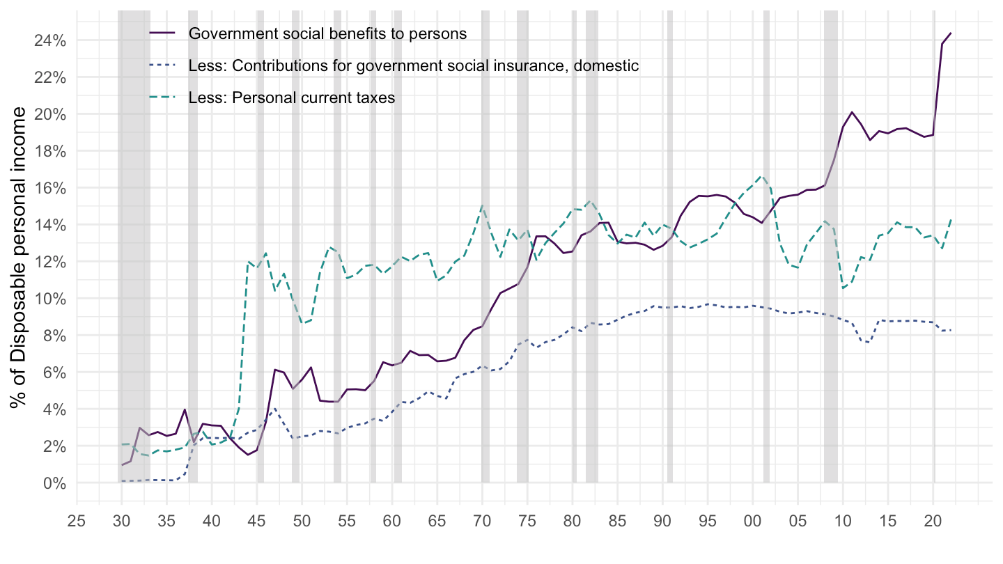

Government social benefits to persons

Code

T20100_A |>
  year_to_date() |>
  group_by(date) |>
  mutate(value = DataValue/DataValue[LineNumber == 27]) |>
  filter(LineNumber %in% c(18:23)) |>
  ggplot() + theme_minimal() + 
  geom_line(aes(x = date, y = value, color = LineDescription, linetype = LineDescription)) +
  theme(legend.title = element_blank(),
        legend.position = c(0.15, 0.8)) +
  geom_rect(data = nber_recessions |>
              filter(Peak > as.Date("1928-01-01")), 
            aes(xmin = Peak, xmax = Trough, ymin = 0, ymax = +Inf), 
            fill = 'grey', alpha = 0.5) + 
  scale_x_date(breaks = seq(1925, 2100, 5) |> paste0("-01-01") |> as.Date(),
               labels = date_format("%Y")) +
  ylab("% of Disposable personal income") + xlab("") +
  scale_color_manual(values = viridis(7)[1:6]) +
  scale_y_continuous(breaks = 0.01*seq(0, 90, 1),
                     labels = scales::percent_format(accuracy = 1))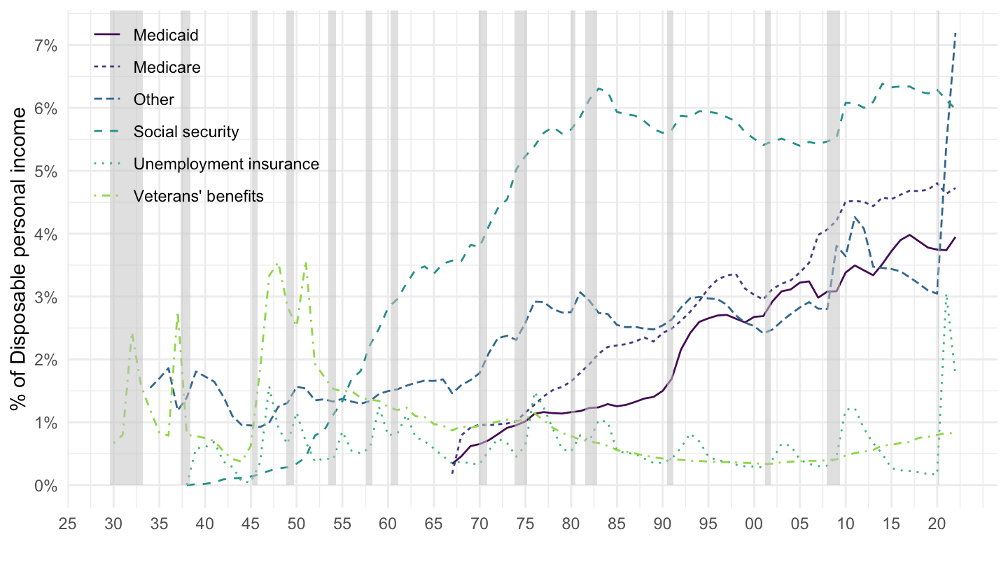

1938, 1958, 1978, 1998, 2018 Table

% of Personal income

Code

T20100_A |>
  year_to_date() |>
  mutate(year = year(date)) |>
  filter(year %in% c(1938, 1958, 1978, 1998, 2018)) |>
  group_by(year) |>
  mutate(value = round(100*DataValue/DataValue[LineNumber == 1], 1)) |>
  ungroup() |>
  select(2, 3, 6, 7) |>
  spread(year, value) %>%
  {if (is_html_output()) datatable(., filter = 'top', rownames = F) else .}

% of Personal Disposable income

Code

T20100_A |>
  year_to_date() |>
  mutate(year = year(date)) |>
  filter(year %in% c(1938, 1958, 1978, 1998, 2018)) |>
  group_by(year) |>
  mutate(value = round(100*DataValue/DataValue[LineNumber == 27], 1)) |>
  ungroup() |>
  select(2, 3, 6, 7) |>
  spread(year, value) %>%
  {if (is_html_output()) datatable(., filter = 'top', rownames = F) else .}

Billions

Code

T20100_A |>
  year_to_date() |>
  mutate(year = year(date)) |>
  filter(year %in% c(1938, 1958, 1978, 1998, 2018)) |>
  group_by(year) |>
  mutate(value = round(DataValue/1000)) |>
  ungroup() |>
  select(2, 3, 6, 7) |>
  spread(year, value) %>%
  {if (is_html_output()) datatable(., filter = 'top', rownames = F) else .}