Scrape using R
R - Code
François Geerolf
Introduction
To create your own datasets, python is particularly useful for scrapping the web, but you can also use R. You will also want to familiarize yourself with regular expressions.
The tidyverse, rvest and janitor packages are needed.
pklist <- c("tidyverse", "rvest", "janitor", "magrittr")
source("https://fgeerolf.com/code/load-packages.R")
read_html is used to transform an html webpage into an html tree (with parents and children), and html_table allows to extract all tables in a webpage.
Price to Rent ratio in U.S. Cities
https://smartasset.com/mortgage/price-to-rent-ratio-in-us-cities
# {html_document}
# <html>
# [1] <head>\n<meta http-equiv="Content-Type" content="text/html; charset=UTF-8 ...
# [2] <body>\n<h1>Index of /emos_prod/reports/public</h1>\n<pre>      <a href=" ...
a_elements <- read_html("https://ec.europa.eu/energy/observatory/reports/") |>
html_elements("a") |>
html_text2()
a_elements# [1] "Name" "Last modified" "Size" "Description"
# [5] "Parent Directory"Most downloaded Songs in the U.K.
https://en.wikipedia.org/wiki/List_of_most-downloaded_songs_in_the_United_Kingdom
data <- "https://en.wikipedia.org/wiki/List_of_most-downloaded_songs_in_the_United_Kingdom" %>%
  read_html %>%
  html_table(header = T, fill = T)
The interesting data is in the second data.frame.
data[[2]][, c(1, 2, 3, 7)] %>%
  as.tibble %>%
  head(10) %>%
{if (is_html_output()) print_table(.) else .}| No. | Artist | Song | Copies sold[a] |
|---|---|---|---|
| 1 | Pharrell Williams | “Happy” | 1,922,000[4] |
| 2 | Adele | “Someone Like You” | 1,637,000+[5] |
| 3 | Robin Thicke featuring T.I. and Pharrell Williams | “Blurred Lines” | 1,620,000+ |
| 4 | Maroon 5 featuring Christina Aguilera | “Moves Like Jagger” | 1,500,000+ |
| 5 | Gotye featuring Kimbra | “Somebody That I Used to Know” | 1,470,000+ |
| 6 | Daft Punk featuring Pharrell Williams | “Get Lucky” | 1,400,000+ |
| 7 | The Black Eyed Peas | “I Gotta Feeling” | 1,350,000+ |
| 8 | Avicii | “Wake Me Up” | 1,340,000+ |
| 9 | Rihanna featuring Calvin Harris | “We Found Love” | 1,337,000+ |
| 10 | Kings of Leon | “Sex on Fire” | 1,293,000+ |
Salaries at U.C. Berkeley, by specialty
http://projects.dailycal.org/paychecker
Using the XML package and the readHTMLTable function, we may download the pays at UC Berkeley, and then plot them by Field.
pays_berkeley <- readHTMLTable("http://projects.dailycal.org/paychecker")[[1]] %>%
  rename(Salary = `Salary (2015)`) %>%
  mutate(Salary = as.numeric(gsub('[$,]', '', Salary)))

pays_berkeley %>%
  head(10) %>%
{if (is_html_output()) print_table(.) else .}| Name | Rank | Department | Salary |
|---|---|---|---|
| Turner, James | Professor | English | 202650 |
| Lee, Taeku | Professor | Political Science | 240691 |
| Jeziorski, Przemyslaw | Assistant Professor | Business | 209741 |
| Rosen, Christine | Associate Professor | Business | 74184 |
| Tang, Maureen | Lecturer | Theater, Dance and Performance Studies | 30931 |
| Barnes, Barbara | Lecturer | Gender and Women’s Studies | 48540 |
| Sankara Rajulu, Bharathy | Lecturer | South & Southeast Asian Studies | 67348 |
| Faber, Benjamin | Assistant Professor | Economics | 189085 |
| Olsen, Carl | Lecturer | Scandinavian Languages | 15663 |
| Foote, Christopher | Lecturer | Business | 18430 |
readHTMLTable("http://projects.dailycal.org/paychecker")[[1]] %>%
  rename(Salary = `Salary (2015)`) %>%
  mutate(Salary = as.numeric(gsub('[$,]', '', Salary))) %>%
  ggplot(., aes(x=Department, y=Salary)) + coord_flip() +
  geom_boxplot(aes(color=Rank,
                     x=reorder(Department, Salary, FUN=max))) +
  scale_y_continuous(labels = scales::dollar) +
  labs(title="Salaries by Department",
       subtitle="UC Berkeley Salaries",
       y="Annual Salary (2015)",
       x="Department") +
  theme(plot.caption = element_text(size=7.5))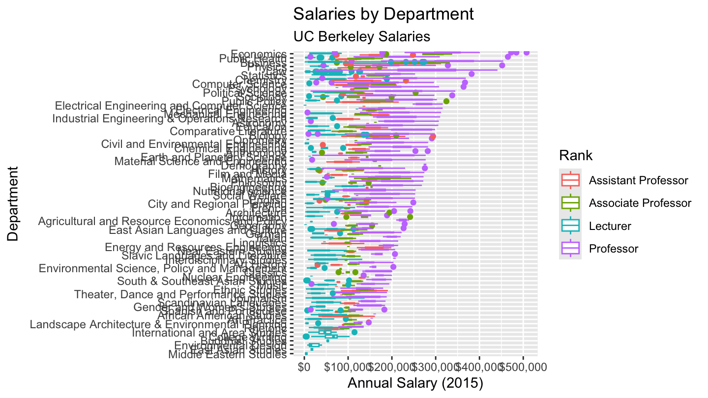