Europe Maps
Code - R
François Geerolf
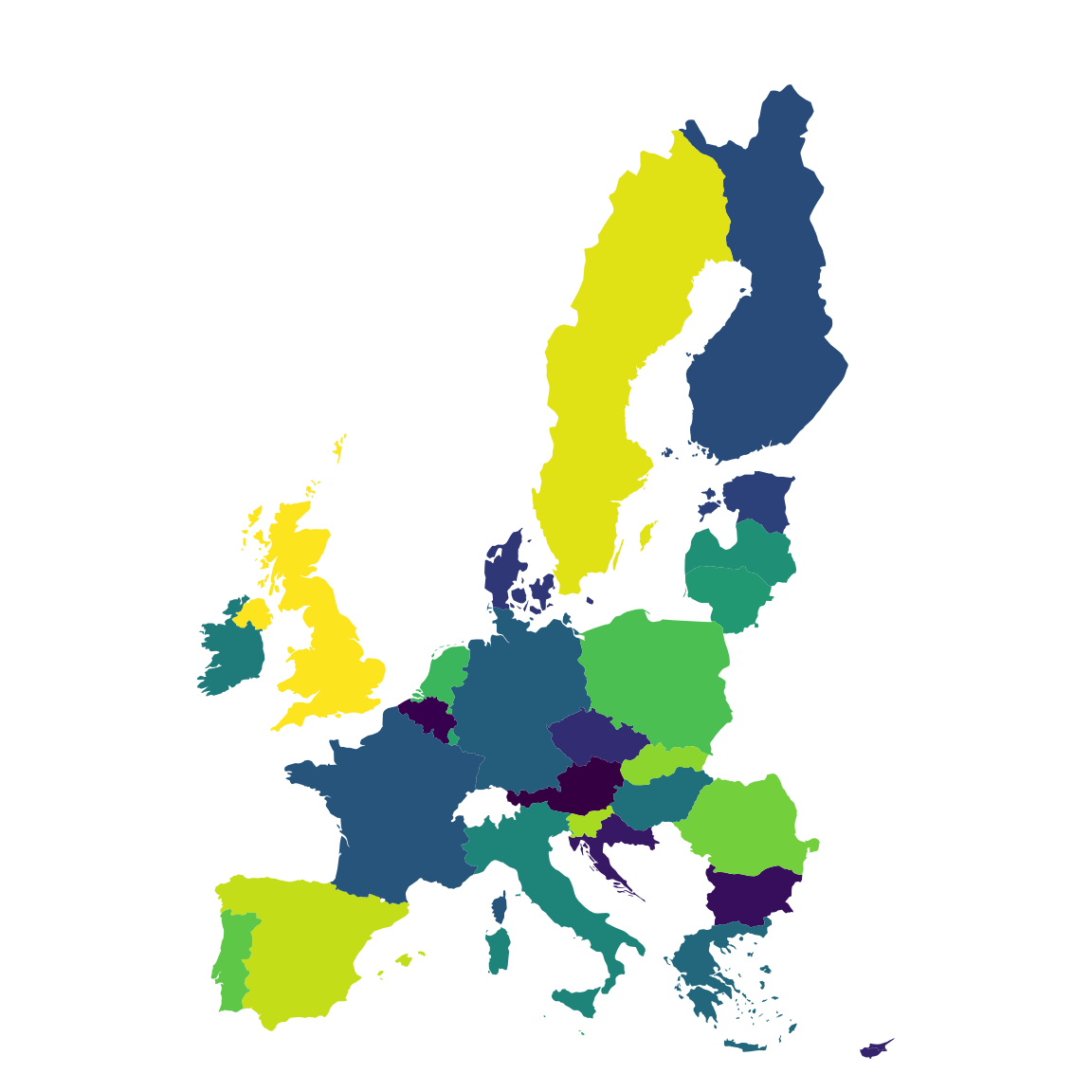
Eurozone
eurozone_centroids <- eurozone %>%
  group_by(region) %>%
  summarise(long = mean(long), lat = mean(lat))

eurozone_centroids %>%
{if (is_html_output()) print_table(.) else .}| region | long | lat |
|---|---|---|
| Austria | 13.473366 | 47.57973 |
| Belgium | 4.732104 | 50.59063 |
| Cyprus | 33.350308 | 35.06384 |
| Estonia | 24.594756 | 58.53494 |
| Finland | 24.430224 | 63.95119 |
| France | 3.226979 | 46.16686 |
| Germany | 10.401156 | 51.20461 |
| Greece | 23.940537 | 38.35875 |
| Ireland | -8.439389 | 53.49476 |
| Italy | 11.752853 | 42.16598 |
| Latvia | 25.369484 | 56.86748 |
| Lithuania | 24.080040 | 55.08304 |
| Luxembourg | 6.062349 | 49.76263 |
| Malta | 14.370850 | 35.96163 |
| Netherlands | 5.322302 | 52.09905 |
| Portugal | -7.887035 | 39.93084 |
| Slovakia | 19.620591 | 48.83819 |
| Slovenia | 14.843692 | 46.12320 |
| Spain | -2.906821 | 40.67995 |
eurozone %>%
  ggplot(., aes(x = long, y = lat)) +
  geom_polygon(aes( group = group, fill = region))+
  geom_text(aes(label = region), data = eurozone_centroids,  size = 3, hjust = 0.5) +
  scale_fill_viridis_d() +
  theme_void()+
  theme(legend.position = "none")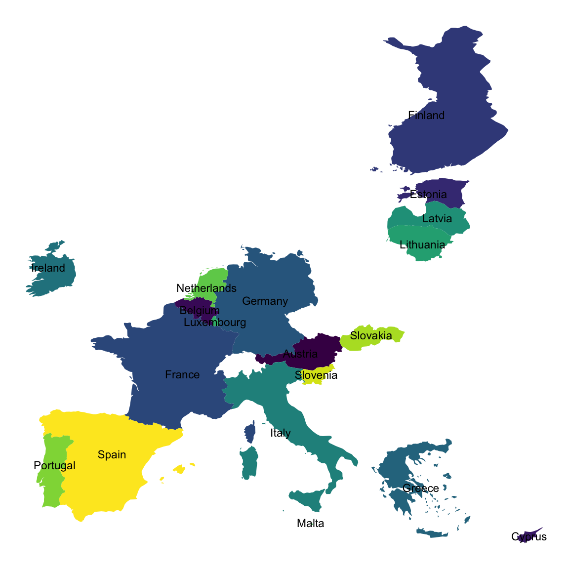
Figure 1: European Map
eurozone %>%
  mutate(lat = case_when(region %in% c("Finland", "Estonia", "Latvia", "Lithuania") ~ lat-10,
                          T ~ lat)) %>%
  ggplot(., aes(x = long, y = lat)) +
  geom_polygon(aes( group = group, fill = region))+
  geom_text(aes(label = region), data = eurozone_centroids %>%
              mutate(lat = case_when(region %in% c("Finland", "Estonia", "Latvia", "Lithuania") ~ lat-10,
                          T ~ lat)),  size = 3, hjust = 0.5) +
  scale_fill_viridis_d() +
  theme_void()+
  theme(legend.position = "none")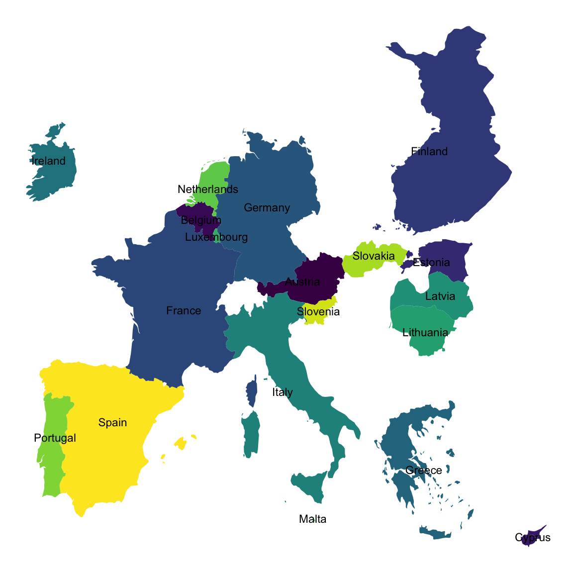
Figure 2: European Map
European Union
european_union_centroids <- european_union %>%
  group_by(region) %>%
  summarise(long = mean(long), lat = mean(lat))

european_union_centroids %>%
{if (is_html_output()) print_table(.) else .}| region | long | lat |
|---|---|---|
| Austria | 13.473366 | 47.57973 |
| Belgium | 4.732104 | 50.59063 |
| Bulgaria | 24.964096 | 42.62486 |
| Croatia | 16.348786 | 44.64204 |
| Cyprus | 33.350308 | 35.06384 |
| Czech Republic | 15.423777 | 49.88404 |
| Denmark | 10.731255 | 55.70473 |
| Estonia | 24.594756 | 58.53494 |
| Finland | 24.430224 | 63.95119 |
| France | 3.226979 | 46.16686 |
| Germany | 10.401156 | 51.20461 |
| Greece | 23.940537 | 38.35875 |
| Hungary | 19.423931 | 47.23226 |
| Ireland | -8.439389 | 53.49476 |
| Italy | 11.752853 | 42.16598 |
| Latvia | 25.369484 | 56.86748 |
| Lithuania | 24.080040 | 55.08304 |
| Luxembourg | 6.062349 | 49.76263 |
| Malta | 14.370850 | 35.96163 |
| Netherlands | 5.322302 | 52.09905 |
| Poland | 19.086516 | 51.40998 |
| Portugal | -7.887035 | 39.93084 |
| Romania | 24.529212 | 45.84465 |
| Slovakia | 19.620591 | 48.83819 |
| Slovenia | 14.843692 | 46.12320 |
| Spain | -2.906821 | 40.67995 |
| Sweden | 17.576305 | 61.89591 |
| UK | -4.098750 | 55.55813 |
european_union %>%
  ggplot(., aes(x = long, y = lat)) +
  geom_polygon(aes( group = group, fill = region))+
  geom_text(aes(label = region), data = european_union_centroids,  size = 3, hjust = 0.5) +
  scale_fill_viridis_d() +
  theme_void()+
  theme(legend.position = "none")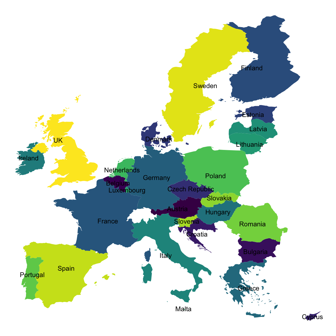
Figure 3: European Map
Europe
europe_centroids <- europe %>%
  group_by(region) %>%
  summarise(long = mean(long), lat = mean(lat))

europe_centroids %>%
{if (is_html_output()) print_table(.) else .}| region | long | lat |
|---|---|---|
| Albania | 20.109251 | 41.09708 |
| Andorra | 1.563245 | 42.52996 |
| Austria | 13.473366 | 47.57973 |
| Belarus | 28.117585 | 53.53241 |
| Belgium | 4.732104 | 50.59063 |
| Bosnia and Herzegovina | 18.134789 | 44.06762 |
| Bulgaria | 24.964096 | 42.62486 |
| Croatia | 16.348786 | 44.64204 |
| Cyprus | 33.350308 | 35.06384 |
| Czech Republic | 15.423777 | 49.88404 |
| Denmark | 10.731255 | 55.70473 |
| Estonia | 24.594756 | 58.53494 |
| Finland | 24.430224 | 63.95119 |
| France | 3.226979 | 46.16686 |
| Germany | 10.401156 | 51.20461 |
| Greece | 23.940537 | 38.35875 |
| Hungary | 19.423931 | 47.23226 |
| Iceland | -19.867290 | 65.30842 |
| Ireland | -8.439389 | 53.49476 |
| Italy | 11.752853 | 42.16598 |
| Kosovo | 20.857038 | 42.58538 |
| Latvia | 25.369484 | 56.86748 |
| Liechtenstein | 9.547135 | 47.14268 |
| Lithuania | 24.080040 | 55.08304 |
| Luxembourg | 6.062349 | 49.76263 |
| Macedonia | 21.649726 | 41.63621 |
| Malta | 14.370850 | 35.96163 |
| Moldova | 28.545301 | 47.06328 |
| Monaco | 7.411649 | 43.75479 |
| Montenegro | 19.257525 | 42.81717 |
| Netherlands | 5.322302 | 52.09905 |
| Norway | 16.243541 | 69.87700 |
| Poland | 19.086516 | 51.40998 |
| Portugal | -7.887035 | 39.93084 |
| Romania | 24.529212 | 45.84465 |
| San Marino | 12.452120 | 43.94140 |
| Serbia | 20.751169 | 44.25245 |
| Slovakia | 19.620591 | 48.83819 |
| Slovenia | 14.843692 | 46.12320 |
| Spain | -2.906821 | 40.67995 |
| Sweden | 17.576305 | 61.89591 |
| Switzerland | 8.312952 | 46.74157 |
| UK | -4.098750 | 55.55813 |
| Ukraine | 31.233695 | 48.47920 |
europe %>%
  ggplot(., aes(x = long, y = lat)) +
  geom_polygon(aes( group = group, fill = region))+
  geom_text(aes(label = region), data = europe_centroids,  size = 3, hjust = 0.5) +
  scale_fill_viridis_d() +
  theme_void()+
  theme(legend.position = "none")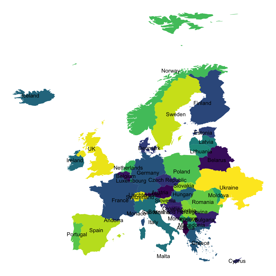
Figure 4: Europe
Example 1: European Union
european_union %>%
  ggplot(., aes(x = long, y = lat, group = group, fill = region)) +
  geom_polygon() + coord_map() +
  scale_fill_viridis_d() +
  theme_void() +
  theme(legend.position = "none")
Example 2: European Union Bigger
Using fig.height = 6, fig.width = 6
european_union %>%
  ggplot(., aes(x = long, y = lat, group = group, fill = region)) +
  geom_polygon() + coord_map() +
  scale_fill_viridis_d() +
  theme_void() +
  theme(legend.position = "none")