R Statistical Software

What is R ? Why is it useful to learn R ?

R is a free software environment for statistical computing and graphics. It is released under the GNU General Public License, and an alternative to other popular commercial softwares such as Stata, or even Microsoft Excel. Many statisticians and data scientists use R (many also use python) for exploring data.

We shall use Intermediate Macroeconomics as an excuse to teach ourselves some elements of R. Macroeconomic data is constantly evolving in real-time, and R allows you to retrieve real-time data from up-to-date sources, as well as work with these datasets, quite easily. Learning a statistical software would also help you think critically about macroeconomic analysis that is typically found in The Economist, the Wall Street Journal, the New York Times, and other reliable sources of information, which often make heavy use of data. R make computations easy (such as transforming values to growth rate), detrending, as well as presenting data in the best way possible (such as plotting the time series of economic quantities, etc.).

Moreover, many companies/universities in the world currently demands graduates with data science skills. Even the consulting and the finance industry increasingly require knowing how to manipulate datasets. I view Intermediate Macroeconomics as an occasion to teach you these general purpose skills (as economists like to call them). Finally, these skills might also prove useful when you take an Econometrics or a Statistics class, in which you will learn more thoroughly the tools of regression analysis (if you have not already).

Downloading R and Rstudio

First you must get the R statistical software, which you may download from the R webpage. The latest release is R version 4.1.2 (Bird Hippie):

For Mac OSX: download here.
For Windows: download here.
For Linux: download here.

Second, unless you are already very familiar with R already and have a strong preference fpr using R from the command line, I recommend you use a Graphical User Interface (GUI) for R such as R Studio. R Studio’s latest release is 2021.09.2-382:

For Mac OSX: download here.
For Windows: download here.
Other: download here

Getting started with “cheatsheets”

Cheatsheets are a great way to get started on R. A list of cheatsheets is available here. The most important cheatsheets are:

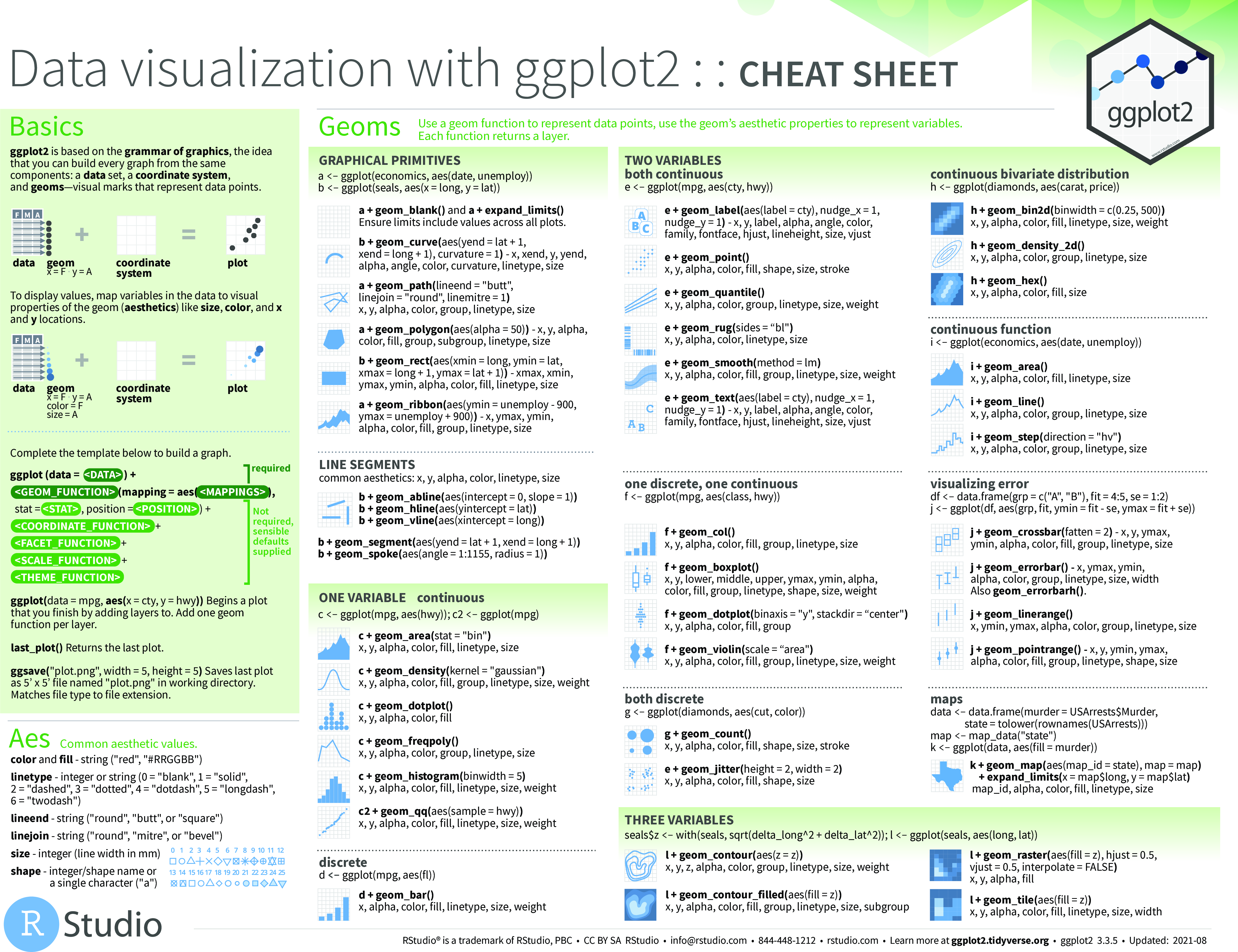
Data transformation with dplyr cheatsheet.
Data visualization with ggplot2 cheatsheet.

Data transformation with `dplyr`

dplyr for data transformation. Note, in particular, the use of pipes %>%: + x %>% f(y) is the same as f(x, y). + y %>% f(x, ., z) is the same as f(x, y, z). + “Piping” with %>% makes code more readable.

Data visualization with `ggplot2` cheatsheet

Examples

# # A tibble: 3 × 2
#   Species      avg
#   <fct>      <dbl>
# 1 versicolor  2.77
# 2 virginica   2.97
# 3 setosa      3.43

Packages

The following packages are particularly useful:

ggplot2 for data visualization. Cheatsheet.
stringr for string manipulation. Cheatsheet. Cheatsheet on Regular Expressions.

In addition to the tidyverse collection of R packages, I also use the following packages:

lubridate for working with dates (very useful in macroeconomics !). Cheatsheet.

tidyverse also contains readr which allows to read in data. Cheatsheet

An example from Lecture 1

NIPA data

The power of R is now illustrated using the first Figure in Lecture 1. Data for GDP is taken from the Bureau of Economic Analysis’s National Income and Product Accounts (NIPA) here and data for Personal Consumption Expenditures is taken from there. Note that the BEA’s website is here, and that you get access to this data clicking on Section 1 - Domestic Product and Income and then on Table 1.1.5. which has Gross Domestic Product (A) (Q) (Annual and Quarterly).

rdb (dbnomics) or fredr (FRED)

However, instead of retrieving this data from the BEA, we use the rdbnomics R-package which retrieves data from this website. You must first install and load this package through the following code:

devtools::install_github("dbnomics/rdbnomics")
pklist <- c("tidyverse", "lubridate", "rdbnomics", "scales", "fredr")
source("https://fgeerolf.com/code/load-packages.R")
load(url("https://fgeerolf.com/data/us/nber_recessions.RData"))
fredr_set_key(fred_key)

Download using `rdb`

rdb(ids = c("BEA/NIPA-T10105/A191RC-A", 
            "BEA/NIPA-T10105/DPCERC-A")) %>%
  glimpse()

# Rows: 186
# Columns: 19
# $ `@frequency`    <chr> "annual", "annual", "annual", "annual", "annual", "ann…
# $ concept         <chr> "gross-domestic-product", "gross-domestic-product", "g…
# $ Concept         <chr> "Gross domestic product", "Gross domestic product", "G…
# $ dataset_code    <chr> "NIPA-T10105", "NIPA-T10105", "NIPA-T10105", "NIPA-T10…
# $ dataset_name    <chr> "Table 1.1.5. Gross Domestic Product - LastRevised: Ja…
# $ FREQ            <chr> "A", "A", "A", "A", "A", "A", "A", "A", "A", "A", "A",…
# $ Frequency       <chr> "Annually", "Annually", "Annually", "Annually", "Annua…
# $ indexed_at      <dttm> 2022-01-28 05:22:49, 2022-01-28 05:22:49, 2022-01-28 …
# $ metric          <chr> "millions-of-current-dollars", "millions-of-current-do…
# $ Metric          <chr> "Millions of current Dollars", "Millions of current Do…
# $ original_period <chr> "1929", "1930", "1931", "1932", "1933", "1934", "1935"…
# $ original_value  <chr> "104556", "92160", "77391", "59522", "57154", "66800",…
# $ period          <date> 1929-01-01, 1930-01-01, 1931-01-01, 1932-01-01, 1933-…
# $ provider_code   <chr> "BEA", "BEA", "BEA", "BEA", "BEA", "BEA", "BEA", "BEA"…
# $ series_code     <chr> "A191RC-A", "A191RC-A", "A191RC-A", "A191RC-A", "A191R…
# $ series_name     <chr> "Gross domestic product (line 1) - Annually", "Gross d…
# $ unit            <chr> "level", "level", "level", "level", "level", "level", …
# $ Unit            <chr> "Level", "Level", "Level", "Level", "Level", "Level", …
# $ value           <dbl> 104556, 92160, 77391, 59522, 57154, 66800, 74241, 8483…

Download using `fredr`

Create an API key first here

map_dfr(c("GDP", "PCE"), fredr) %>%
  glimpse()

# Rows: 1,060
# Columns: 5
# $ date           <date> 1946-01-01, 1946-04-01, 1946-07-01, 1946-10-01, 1947-0…
# $ series_id      <chr> "GDP", "GDP", "GDP", "GDP", "GDP", "GDP", "GDP", "GDP",…
# $ value          <dbl> NA, NA, NA, NA, 243.164, 245.968, 249.585, 259.745, 265…
# $ realtime_start <date> 2022-02-14, 2022-02-14, 2022-02-14, 2022-02-14, 2022-0…
# $ realtime_end   <date> 2022-02-14, 2022-02-14, 2022-02-14, 2022-02-14, 2022-0…

mutate, select

rdb(ids = c("BEA/NIPA-T10105/A191RC-A", 
            "BEA/NIPA-T10105/DPCERC-A")) %>%
  mutate(value = value / 1000000,
         series_name = series_name %>% gsub(" - Annually", "", .)) %>%
  select(date = period, value, series_name) %>%
  glimpse()

# Rows: 186
# Columns: 3
# $ date        <date> 1929-01-01, 1930-01-01, 1931-01-01, 1932-01-01, 1933-01-0…
# $ value       <dbl> 0.104556, 0.092160, 0.077391, 0.059522, 0.057154, 0.066800…
# $ series_name <chr> "Gross domestic product (line 1)", "Gross domestic product…

Simple `ggplot2`

rdb(ids = c("BEA/NIPA-T10105/A191RC-A", 
            "BEA/NIPA-T10105/DPCERC-A")) %>%
  mutate(value = value / 1000000,
         series_name = series_name %>% gsub(" - Annually", "", .)) %>%
  select(date = period, value, series_name) %>%
  ggplot(.) + xlab("") + ylab("Trillion") + theme_minimal() +
  geom_line(aes(x = date, y = value, linetype = series_name)) +
  scale_y_continuous(breaks = seq(0, 20, 2.5),
                     labels = scales::dollar_format(accuracy = 0.1))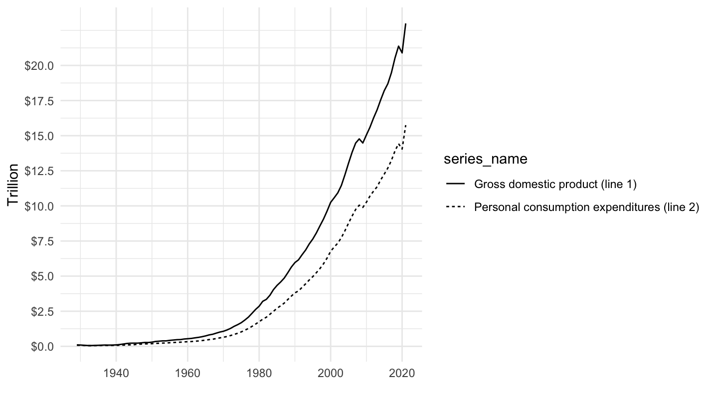

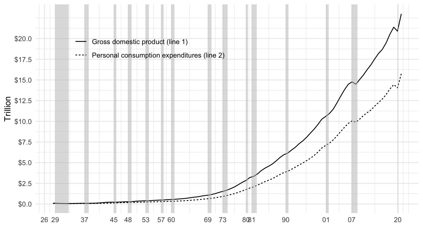
Pretty `ggplot2`

The pretty graph looks like this:

rdb(ids = c("BEA/NIPA-T10105/A191RC-A", 
            "BEA/NIPA-T10105/DPCERC-A")) %>%
  mutate(value = value / 1000000,
         series_name = series_name %>% gsub(" - Annually", "", .)) %>%
  select(date = period, value, series_name) %>%
  ggplot(.) + 
  geom_line(aes(x = date, y = value, linetype = series_name)) + theme_minimal() +
  geom_rect(data = nber_recessions %>%
              filter(Peak > as.Date("1928-01-01")), 
            aes(xmin = Peak, xmax = Trough, ymin = -Inf, ymax = +Inf), 
            fill = 'grey', alpha = 0.5) + 
  theme(legend.title = element_blank(),
        legend.position = c(0.3, 0.8)) +
  scale_x_date(breaks = nber_recessions$Peak,
               labels = date_format("%y")) +
  xlab("") + ylab("Trillion") +
  scale_y_continuous(breaks = seq(0, 20, 2.5),
                     labels = scales::dollar_format(accuracy = 0.1))

R Statistical Software - An Introduction

R - Code

François Geerolf

R Statistical Software

What is R ? Why is it useful to learn R ?

Downloading R and Rstudio

Getting started with “cheatsheets”

Data transformation with `dplyr`

Data visualization with `ggplot2` cheatsheet

Examples

Packages

An example from Lecture 1

NIPA data

rdb (dbnomics) or fredr (FRED)

Download using `rdb`

Download using `fredr`

mutate, select

Simple `ggplot2`

Pretty `ggplot2`

R Statistical Software - An Introduction

R - Code

François Geerolf

R Statistical Software

What is R ? Why is it useful to learn R ?

Downloading R and Rstudio

Getting started with “cheatsheets”

Data transformation with dplyr

Data visualization with ggplot2 cheatsheet

Examples

Packages

An example from Lecture 1

NIPA data

rdb (dbnomics) or fredr (FRED)

Download using rdb

Download using fredr

mutate, select

Simple ggplot2

Pretty ggplot2

Data transformation with `dplyr`

Data visualization with `ggplot2` cheatsheet

Download using `rdb`

Download using `fredr`

Simple `ggplot2`

Pretty `ggplot2`