Get Started
Code - R
François Geerolf
“Programs must be written for people to read and only incidentally for machines to execute.” (Hal Abelson)
Getting started with R
Downloading
You need to install R and Rstudio:
You can get R statistical software on the UCLA mirror here.
I recommend you use a Graphical User Interface (GNU) for R such as R Studio. You can get the latest release here: download here.
R or Stata?
In my opinion, R is better than Stata for tidying data: preparing, merging, exploring. For regressions Stata is perhaps marginally better, just because more economists (still) use it. Also, R is for geeks. Can you do that in Stata?
# [1] I II III IV V X L C M MMIntroduction to R
I recommend cheatsheets to get started on R. Many are available, but the 2 main cheatsheets are:
R for Stata users
For Stata users, here are resources to get you started in R:
Advanced R
Here are more advanced resources:
- R for data science, by Garrett Grolemund and Hadley Wickham.
- R Markdown: The Definitive Guide, by Yihui Xie, J. J. Allaire, Garrett Grolemund.
- bookdown: Authoring Books and Technical Documents with R Markdown, by Yihui Xie.
- Datacamp also has great learning tools for
R, as well asPython.
Packages (Libraries)
Once you have installed some packages, don’t forget to update them from time to time typing update.packages(ask=FALSE).
Necessary
I will mostly be using tidyverse, from Hadley Wickham, for data manipulation as well as plotting data. This cheatsheet has a beginner’s introduction to tidyverse, and tidyverse is presented on this blogpost. tidyverse is a powerful collection of R packages that are data tools for transforming and visualizing data. Datacamp has a free tutorial for tidyverse, which can get you started. The following packages are particularly useful:
dplyrfor data manipulation. Cheatsheet. You will find a tutorial in 4 parts here: Part 1 / Part 2 / Part 3 / Part 4. Note, in particular, the use of pipes %>%:- x %>% f(y) is the same as f(x, y).
- y %>% f(x, ., z) is the same as f(x, y, z).
“Piping” with %>% makes code more readable. For example, the following code computes an average of
Sepal.WidthbySpeciesin theirisdatabase, and then orders the Species by their averageSepal.Width. More generally, instead of writing \(i(h(g(f())))\) which is very hard to read when \(f\), \(g\), \(h\) and \(i\) are complex functions, pipes allow you to write functions in the order they are being called: x %>% f %>% g %>% h %>% i. Try it !
# # A tibble: 3 x 2 # Species avg # <fct> <dbl> # 1 versicolor 2.77 # 2 virginica 2.97 # 3 setosa 3.43ggplot2for data visualization. Cheatsheet. Combined withtidyverse,ggplot2proves very powerful.stringrfor string manipulation. A cheatsheet is available here.str_replace_all("Fifty states, three thousand counties", c("Fifty" = "50", "three thousand" = "3000"))# [1] "50 states, 3000 counties"If you do want to work on string variables a lot, for example to do web scrapping, then you should learn about regular expressions.
readrto read in data. A cheatsheet is provided here.
In addition to the tidyverse collection of R packages, I also use the following packages:
broomfor bringing the modeling process into a tidy workflow. A presentation is available here. There are 3 main functions:tidy: estimates, standard errors, confidence intervals, etc.augment: residuals, fitted values, influence measures, etc.glance: whole-model summaries: AIC, R-squared, etc.
lubridatefor working with dates (very useful in macroeconomics !). A cheatsheet is provided here.
Other
Here are other potentially useful packages:
tidytextfor analyzing text with thetidyversetools. A great introduction to this package is provided here.
bookdownas a great complement to R-markdown, in order to write more advanced documents. A great introduction is also provided here.DTfor displaying Tables in Javascript, as here. An introduction is provided here.
Graphing
Scales
To add tickers with percentage:
fredr(series_id = "FYOIGDA188S") %>%
  mutate(value = value / 100) %>%
  ggplot(data = ., mapping = aes(x = date, y = value)) + geom_line() +
  labs(x = "Observation Date", y = "Rate") + theme_minimal() +
  scale_x_date(breaks = as.Date(paste0(seq(1920, 2020, 10), "-01-01")),
               labels = date_format("%y")) +
  scale_y_continuous(breaks = 0.01*seq(-1, 3.5, 0.25),
                     labels = scales::percent_format(accuracy = 0.05)) +
  xlab("") + ylab("")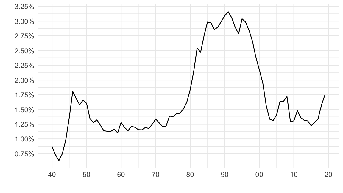
Figure 1: U.S. Interest Payments as a % of GDP (Source: FRED).
Colors
Computers are about representing data using bits. Colors are no exception. A color can be represented as a sum of Red, Green, and Blue. These levels are coded using \(8\) bits, so there are \(2^8=256\) levels of colors. One way to represent these \(256\) levels is to use hexadecimal notation (numbers \(0-9\), and letters A-F, so \(16\) possibilities), with \(2\) characters: \(16^2=256\).
Here is a cheatsheet with a list of colors.
Below is a visualization of the RGB additive color model with ggplot2.
expand.grid(r = seq(0, 1, 0.1), g = seq(0, 1, 0.1), b = seq(0, 1, 0.1)) %>%
  ggplot() + facet_wrap( ~ paste0("Blue: ", b)) +
  scale_x_continuous(name = "Red",
                     breaks = seq(0.05, 1.05, 0.2),
                     labels = seq (0, 1, 0.2)) +
  scale_y_continuous(name = "Green",
                     breaks = seq(0.05, 1.05, 0.2),
                     labels = seq(0, 1, 0.2)) +
  scale_fill_identity() +
  geom_rect(aes(xmin = r, xmax = r + resolution(r),
                ymin = g, ymax = g + resolution(g),
                fill = rgb(r, g, b)),
            color = "white", size = 0.1)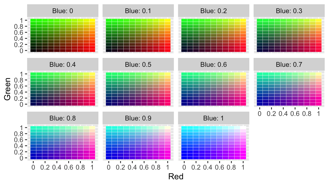
Figure 2: RGB Additive Color Model: By Levels of Blue (0 to 1)
df <- data.frame(a = 3, x = 1:256)
bar_plot <- function(df) {
  barplot(height = df[["a"]], col = df[["col"]], border = NA, space = 0, yaxt = 'n')
}
df$col <- colour_values(df$x, palette = "viridis")
bar_plot(df)
Figure 3: Viridis Colors
Maps
To plot our first map, we use 2000 census county-level data on median rents. First, load tidycensus as well as choroplethr. Second, get a key for the Census API here, input it to census_key, and run the following in a R chunk:
Finally, plot median rents by county in the 2000 Census:
get_decennial(geography = "county", variables = "H063001", year = 2000) %>%
  mutate(region = GEOID %>% as.numeric) %>%
  mutate(value = case_when(value < 200 ~ "$0 to $200",
                           value >= 200 & value < 300 ~ "$200 to $300",
                           value >= 300 & value < 400 ~ "$300 to $400",
                           value >= 400 & value < 600 ~ "$400 to $600",
                           value >= 600 & value < 800 ~ "$600 to $800",
                           value >= 800 ~ "$800+")) %>%
  filter(!is.na(value)) %>%
  county_choropleth() + scale_fill_viridis_d()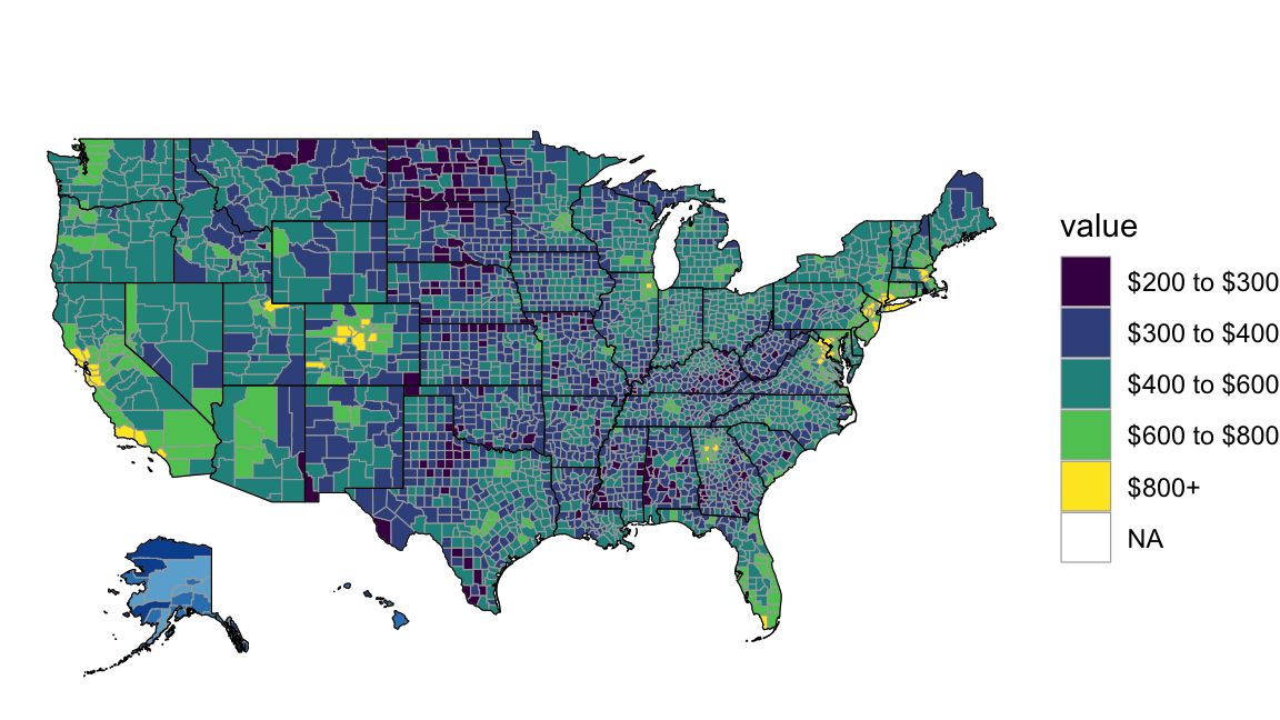
Figure 4: Census-Level Median Rent (Source: 2000 Census)
Dynamic Content
R-markdown allows to create dynamic content inside html files, such as the below map.
Or the below time series of Bitcoin prices.
Or a chart of stock prices:
options("getSymbols.warning4.0" = FALSE)
options("getSymbols.yahoo.warning" = FALSE)
x <- getSymbols("GOOG", auto.assign = FALSE)
y <- getSymbols("AMZN", auto.assign = FALSE)

highchart(type = "stock") %>%
  hc_add_series(x) %>%
  hc_add_series(y, type = "ohlc")
Or a map of county-level unemployment.
data(unemployment)

hcmap("countries/us/us-all-all", data = unemployment,
      name = "Unemployment", value = "value", joinBy = c("hc-key", "code"),
      borderColor = "transparent") %>%
  hc_colorAxis(dataClasses = color_classes(c(seq(0, 10, by = 2), 50))) %>%
  hc_legend(layout = "vertical", align = "right",
            floating = TRUE, valueDecimals = 0, valueSuffix = "%")
mapdata <- get_data_from_map(download_map_data("countries/us/us-all"))
set.seed(1234)
data_fake <- mapdata %>%
select(code = `hc-a2`) %>%
mutate(value = 1e5 * abs(rt(nrow(.), df = 10)))
hcmap("countries/us/us-all", data = data_fake, value = "value",
joinBy = c("hc-a2", "code"), name = "Fake data",
dataLabels = list(enabled = TRUE, format = '{point.name}'),
borderColor = "#FAFAFA", borderWidth = 0.1,
tooltip = list(valueDecimals = 2, valuePrefix = "$", valueSuffix = " USD")) Regressions
Ordinary Least Squares
IV Regression
# For Card's data, fit an IV model of log wage on the treatment variable (education)
# using the IV nearc4, with measured covariates (included exogenous variables)
# exper, expersq, black, south, smsa, smsa66
data(card.data)
ivmodel = ivreg(lwage ~ educ + exper + expersq + black + south + smsa + smsa66,
              ~ nearc4 + exper + expersq + black + south + smsa + smsa66,
              x = TRUE, data = card.data)
ivmodel %>%
  summary
#
# Call:
# ivreg(formula = lwage ~ educ + exper + expersq + black + south +
# smsa + smsa66 | nearc4 + exper + expersq + black + south +
# smsa + smsa66, data = card.data, x = TRUE)
#
# Residuals:
# Min 1Q Median 3Q Max
# -1.76404 -0.22980 0.02407 0.24842 1.40655
#
# Coefficients:
# Estimate Std. Error t value Pr(>|t|)
# (Intercept) 3.9768461 0.8988599 4.424 1.00e-05 ***
# educ 0.1187744 0.0534800 2.221 0.0264 *
# exper 0.1019455 0.0229290 4.446 9.06e-06 ***
# expersq -0.0022778 0.0003285 -6.933 5.02e-12 ***
# black -0.1429037 0.0560350 -2.550 0.0108 *
# south -0.1083667 0.0235244 -4.607 4.26e-06 ***
# smsa 0.1266673 0.0294666 4.299 1.77e-05 ***
# smsa66 0.0173992 0.0217012 0.802 0.4228
# ---
# Signif. codes: 0 '***' 0.001 '**' 0.01 '*' 0.05 '.' 0.1 ' ' 1
#
# Residual standard error: 0.3842 on 3002 degrees of freedom
# Multiple R-Squared: 0.2522, Adjusted R-squared: 0.2504
# Wald test: 107.5 on 7 and 3002 DF, p-value: < 2.2e-16# [1] "Cluster Robust Standard Errors"#
# t test of coefficients:
#
# Estimate Std. Error t value Pr(>|t|)
# (Intercept) 3.97684608 0.83943970 4.7375 2.264e-06 ***
# educ 0.11877444 0.05022730 2.3647 0.018106 *
# exper 0.10194549 0.01850452 5.5092 3.909e-08 ***
# expersq -0.00227778 0.00041633 -5.4711 4.840e-08 ***
# black -0.14290368 0.04585875 -3.1162 0.001849 **
# south -0.10836674 0.04309316 -2.5147 0.011965 *
# smsa 0.12666726 0.02848766 4.4464 9.049e-06 ***
# smsa66 0.01739923 0.02062639 0.8435 0.398993
# ---
# Signif. codes: 0 '***' 0.001 '**' 0.01 '*' 0.05 '.' 0.1 ' ' 1Details
- Tidy, Augment and Glance:
tidy,augmentandglance. html